Lasso vs Ridge vs Elastic Net | ML
Last Updated :
10 Jan, 2023
Bias:
Biases are the underlying assumptions that are made by data to simplify the target function. Bias does help us generalize the data better and make the model less sensitive to single data points. It also decreases the training time because of the decrease in complexity of target function High bias suggest that there is more assumption taken on target function. This leads to the underfitting of the model sometimes.
Examples of High bias Algorithms include Linear Regression, Logistic Regression etc.
Variance:
In machine learning, Variance is a type of error that occurs due to a model’s sensitivity to small fluctuations in the dataset. The high variance would cause an algorithm to model the outliers/noise in the training set. This is most commonly referred to as overfitting. In this situation, the model basically learns every data point and does not offer good prediction when it tested on a novel dataset.
Examples of High variance Algorithms include Decision Tree, KNN etc.
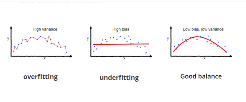
Overfitting vs Underfitting vs Just Right
Let’s consider a simple regression model that aims to predict a variable Y, from the linear combination of variables X and a normally distributed error term


where

is the normal distribution that adds some noise in the prediction.
Here

is the vector representing the coefficient of variables in the X that we need to estimate from the training data. We need to estimate them in such a way that it produces the lowest residual error. This error is defined as:

To calculate

we use the following matrix transformation.

Here Bias and Variance of
can be defined as:

and

We can simplify the error term of the OLS equation defined above in terms of bias and variance as follows:

The first term of above equation represents
Bias2. The second term represents
Variance and the third term (

) is unreducible error term.

Variance/ Bias vs Error
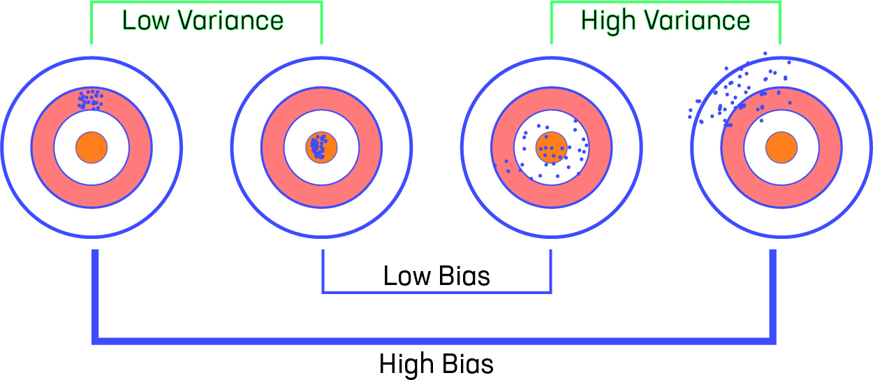
Variance-Bias-Visualization
Let us consider that we have a very accurate model, this model has a low error in predictions and it’s not from the target (which is represented by bull’s eye). This model has low bias and variance. Now, if the predictions are scattered here and there then that is the symbol of high variance, also if the predictions are far from the target then that is the symbol of high bias.
Sometimes we need to choose between low variance and low bias. There is an approach that prefers some bias over high variance, this approach is called
Regularization. It works well for most of the classification/regression problems.
Ridge Regression :
In Ridge regression, we add a penalty term which is equal to the square of the coefficient. The
L2 term is equal to the square of the magnitude of the coefficients. We also add a coefficient

to control that penalty term. In this case if
is zero then the equation is the basic OLS else if

then it will add a constraint to the coefficient. As we increase the value of

this constraint causes the value of the coefficient to tend towards zero. This leads to tradeoff of higher bias (dependencies on certain coefficients tend to be 0 and on certain coefficients tend to be very large, making the model less flexible) for lower variance.

where
is regularization penalty.
Limitation of Ridge Regression: Ridge regression decreases the complexity of a model but does not reduce the number of variables since it never leads to a coefficient been zero rather only minimizes it. Hence, this model is not good for feature reduction.
Lasso Regression :
Lasso regression stands for Least Absolute Shrinkage and Selection Operator. It adds penalty term to the cost function. This term is the absolute sum of the coefficients. As the value of coefficients increases from
0 this term penalizes, cause model, to decrease the value of coefficients in order to reduce loss. The difference between ridge and lasso regression is that it tends to make coefficients to absolute zero as compared to Ridge which never sets the value of coefficient to absolute zero.
 Limitation of Lasso Regression:
- Lasso sometimes struggles with some types of data. If the number of predictors (p) is greater than the number of observations (n), Lasso will pick at most n predictors as non-zero, even if all predictors are relevant (or may be used in the test set).
- If there are two or more highly collinear variables then LASSO regression select one of them randomly which is not good for the interpretation of data
Elastic Net :
Sometimes, the lasso regression can cause a small bias in the model where the prediction is too dependent upon a particular variable. In these cases, elastic Net is proved to better it combines the regularization of both lasso and Ridge. The advantage of that it does not easily eliminate the high collinearity coefficient.
 Reference – Elastic Net Paper
Please Login to comment...