Time Series Decomposition Techniques

Time series data consists of observations taken at consecutive points in time. These data can often be decomposed into multiple components to better understand the underlying patterns and trends. Time series decomposition is the process of separating a time series into its constituent components, such as trend, seasonality, and noise. In this article, we will explore various time series decomposition techniques, their types, and provide code samples for each.

Time series decomposition helps us break down a time series dataset into three main components:

1. Trend: The trend component represents the long-term movement in the data, representing the underlying pattern.
2. Seasonality: The seasonality component represents the repeating, short-term fluctuations caused by factors like seasons or cycles.
3. Residual (Noise): The residual component represents random variability that remains after removing the trend and seasonality.

By separating these components, we can gain insights into the behavior of the data and make better forecasts.

Types of Time Series Decomposition Techniques

Additive Decomposition:

• In additive decomposition, the time series is expressed as the sum of its components:
• It’s suitable when the magnitude of seasonality doesn’t vary with the magnitude of the time series.
  

Multiplicative Decomposition:

• In multiplicative decomposition, the time series is expressed as the product of its components:
• It’s suitable when the magnitude of seasonality scales with the magnitude of the time series.

Methods of Decomposition

Moving Averages:

• Moving averages involve calculating the average of a certain number of past data points.
• It helps smooth out fluctuations and highlight trends.

Seasonal Decomposition of Time Series

• The Seasonal and Trend decomposition using Loess (STL) is a popular method for decomposition, which uses a combination of local regression (Loess) to extract the trend and seasonality components.

Exponential Smoothing State Space Model

• This method involves using the ETS framework to estimate the trend and seasonal components in a time series.

Implementation in Python

Let’s go through an example of applying multiple time series decomposition techniques to a sample dataset. We’ll use Python and some common libraries.

Step 1: Import the required libraries.

We have imported the following libraries:

• NumPy for numeric computing and for scientific and data analysis tasks, offering high-performance array operations and mathematical capabilities.
• Pandas for data manipulation and analysis library.
• Matplotlib is a versatile library for creating static, animated, or interactive visualizations
• Statsmodels Time Series Analysis (tsa) Module
  • The Statsmodels library is used for estimating and interpreting various statistical models in Python.
  • The tsa module within Statsmodels focuses on time series analysis and provides tools for decomposing time series, fitting models, and conducting statistical tests for time series data.
  • It is widely used for time series forecasting, econometrics, and statistical analysis of temporal data.

Step 2: Create a Synthetic Time Series Dataset

The following generates a synthetic time series dataset (ts) with daily data points that combine a sine wave pattern and random noise, simulating a time series with some underlying periodic behavior and variability. The time series spans one year, from “2021-01-01” to the end of the year. The random seed is set to ensure reproducibility.

Output:

2021-01-01    0.882026
2021-01-02    0.217292
2021-01-03    0.523791
2021-01-04    1.172066
2021-01-05    1.002581
                ...   
2021-12-27    0.263264
2021-12-28   -0.066917
2021-12-29    0.414305
2021-12-30    0.135561
2021-12-31   -0.025054
Freq: D, Length: 365, dtype: float64

Step 3: Visualize the Dataset

The following code creates a line plot of the original time series (ts) and sets up the plot with specific dimensions. It also adds a legend to the plot to label the time series data, making it more informative and easier to understand when interpreting the visualization. The resulting plot will display the time series data over time, with dates on the x-axis and the values on the y-axis.

Output:

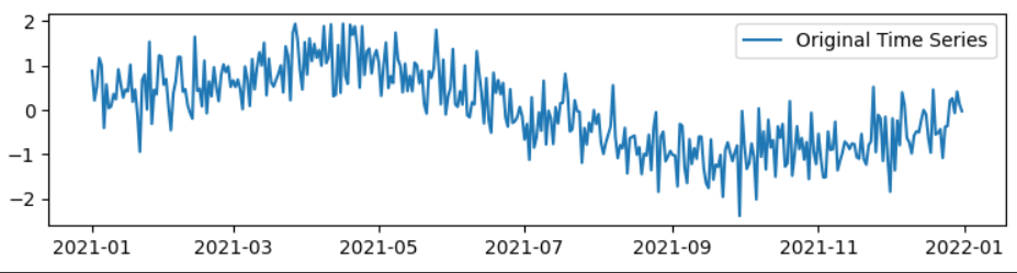
Generated Time Series

Step 3: Apply Additive Decomposition

The following code uses the seasonal_decomposition function from the Statsmodels library to decompose the original time series (ts) into its constituent components using an additive model.

Syntax of seasonal_decompose is provided below:

seasonal_decompose(x, model='additive', filt=None, period=None, two_sided=True, extrapolate_trend=0)

We can also set model=’multiplicative’ but, our data contains zero and negative values. Hence, we are only going to proceed with the additive model.

The code performs an additive decomposition of the original time series and stores the result in the result_add variable, allowing you to further analyze and visualize the decomposed components.

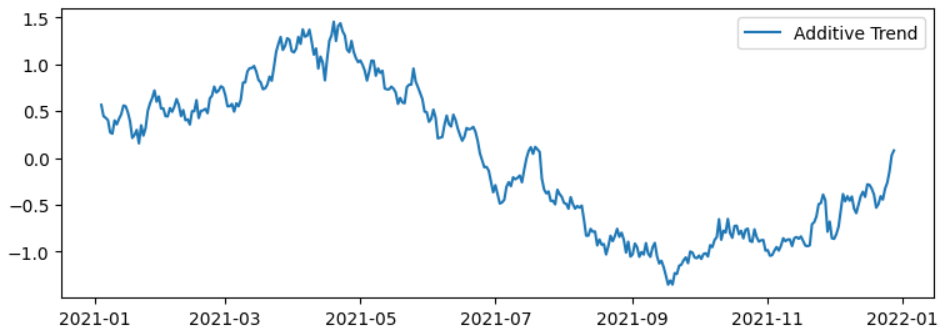
Step 4: Plot the trend component

The following code creates a line plot of the trend component obtained from the additive decomposition of the time series and sets up the plot with specific dimensions. It also adds a legend to the plot to label the trend component, making it more informative and easier to understand when interpreting the visualization. The resulting plot will display the trend component of the time series over time.

Output:

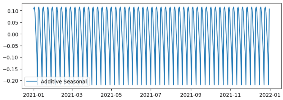
Step 5: Plot the seasonal component

The following code creates a line plot of the seasonal component obtained from the additive decomposition of the time series and sets up the plot with specific dimensions. It also adds a legend to the plot to label the seasonal component, making it more informative and easier to understand when interpreting the visualization. The resulting plot will display the seasonal component of the time series over time.

Output:

Step 6: Calculate the Simple Moving Average (SMA)

The provided code calculates a simple moving average (SMA) for the original time series ts with a 7-day moving window

Output:

2021-01-01         NaN
2021-01-02         NaN
2021-01-03         NaN
2021-01-04         NaN
2021-01-05         NaN
                ...   
2021-12-27   -0.326866
2021-12-28   -0.262944
2021-12-29   -0.142060
2021-12-30    0.030998
2021-12-31    0.081171
Freq: D, Length: 365, dtype: float64

Step 7: Calculate Exponential Moving Average (EMA)

The provided code calculates an exponential moving average (EMA) for the original time series ts with a 30-day window.

Output:

2021-01-01    0.882026
2021-01-02    0.839140
2021-01-03    0.818795
2021-01-04    0.841587
2021-01-05    0.851973
                ...   
2021-12-27   -0.428505
2021-12-28   -0.405176
2021-12-29   -0.352307
2021-12-30   -0.320831
2021-12-31   -0.301749
Freq: D, Length: 365, dtype: float64

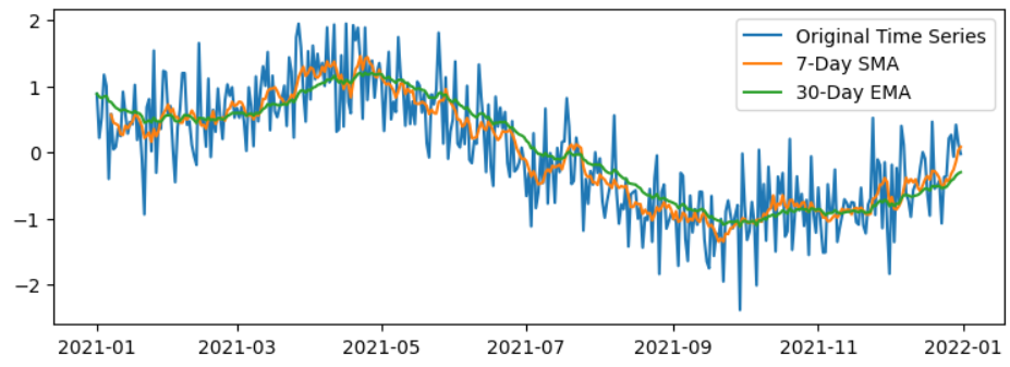
Step 8: Plotting the Moving Averages

The provided code is responsible for creating a plot that overlays the original time series (ts) with both the 7-day simple moving average (SMA) and the 30-day exponential moving average (EMA).components:

Output:

Conclusion

Time series decomposition is a crucial step in understanding and analyzing time series data. By breaking down a time series into its trend, seasonality, and residual components, we can gain valuable insights for forecasting, anomaly detection, and decision-making. Depending on the nature of your data, you can choose between additive and multiplicative decomposition methods. Additionally, moving averages can be a useful tool for smoothing out data and simplifying complex patterns. These techniques are essential for anyone working with time series data, from financial analysts to data scientists, and can lead to more accurate predictions and better-informed decisions.