Analyzing Decision Tree and K-means Clustering using Iris dataset

Iris Dataset is one of best know datasets in pattern recognition literature. This dataset contains 3 classes of 50 instances each, where each class refers to a type of iris plant. One class is linearly separable from the other 2 the latter are NOT linearly separable from each other.

Attribute Information:

1. Sepal Length in cm
2. Sepal Width in cm
3. Petal Length in cm
4. al Width in cm
5. Class:
   • Iris Setosa
   • Iris Versicolour
   • Iris Virginica

Let’s perform Exploratory data analysis on the dataset to get our initial investigation right.

Importing Libraries and Dataset

Python libraries make it very easy for us to handle the data and perform typical and complex tasks with a single line of code.

• Pandas: This library helps to load the data frame in a 2D array format and has multiple functions to perform analysis tasks in one go.
• Numpy: Numpy arrays are very fast and can perform large computations in a very short time.
• Matplotlib/Seaborn: This library is used to draw visualizations.
• Sklearn: This module contains multiple libraries having pre-implemented functions to perform tasks from data preprocessing to model development and evaluation.

Now let’s load the dataset from sklearn.datasets and seaborn.

Output:

Output:

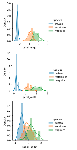
Distribution plot for the features of the three classes available in the dataset three classes

Insights from EDA:

1. It seems feature Petal length properly differentiates  classes
2. Hence  feature importance of petal length should be more

Decision Tree Algorithm with Iris Dataset

A Decision Tree  is one of the popular algorithms for classification and prediction tasks and also a supervised machine learning algorithm

• It begins with all elements E as the root node.
• On each iteration of the algorithm, it iterates through the very unused attribute of the set E and calculates (Entropy(H) or Gini Impurity) and Information gain(IG) of this attribute.
• It then selects the attribute which has the smallest Gini Impurity or Largest Information gain.
• The set E is then split by the selected attribute to produce a subset of the data.
• The algorithm continues to recur on each subset, considering only attributes never selected before.
• This depth of the tree stops once we get all nodes as pure nodes.

Now let’s check the performance of the Decision tree model.

Output:

0.98
              precision    recall  f1-score   support

           0       1.00      1.00      1.00        19
           1       1.00      0.94      0.97        16
           2       0.94      1.00      0.97        15

    accuracy                           0.98        50
   macro avg       0.98      0.98      0.98        50
weighted avg       0.98      0.98      0.98        50

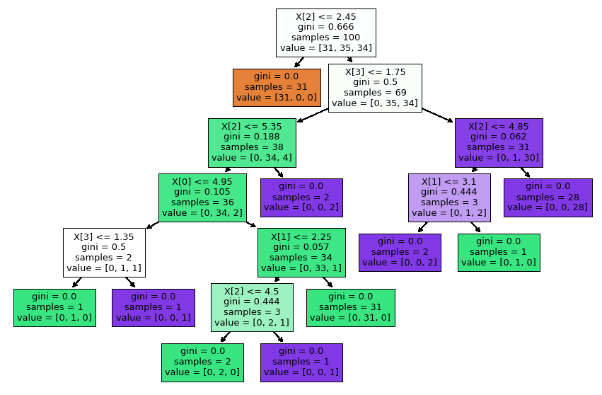
Analyzing Decision Tree formed by the model

One of the advantages of using decision trees over other models is decision trees are highly interpretable and feature selection is automatic hence proper analysis can be done on decision trees. By seeing the above tree we can interpret that.

• If petal_length<2.45 then the output class will always be setosa.
• After depth=2 we can see that we are doing unnecessary splitting because that would just lead to an increase in the variance of the model and thus overfitting.
• After depth=2 majority class of flowers are Versicolor and on the right-hand side of the tree, the majority are virginica.
• Hence there is no need of splitting after depth=2 as it would just lead to overfitting of the model

KMeans Clustering with Iris Dataset

 K-means clustering is an Unsupervised machine learning algorithm. 

• First, choose the clusters K
• Randomly select k centroids from the whole dataset
• Assign all points to the closest cluster centroid
• Recompute centroids again for new clusters
• now repeat steps 3 and 4 until centroids converge

In the above code, we have used the elbow method to get the optimized value of k. If we plot a graph for it we get a value of 3.

Visualizing the Clusters

Output:

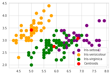
Clusters obtained by using the K-means algorithm

Accuracy and Performance of Model

Now let’s check the performance of the model.

Output:

 

As the algorithm is an unsupervised algorithm we don’t have test data here to check the performance of the model on it. Setosa class is clustered perfectly. While Versicolor has only 2 misclassifications.  Class virginica is getting overlapped Versicolor hence there is 14 misclassifications.