Contrastive Learning In NLP

Last Updated : 29 Oct, 2021

The goal of contrastive learning is to learn such embedding space in which similar samples are close to each other while dissimilar ones are far apart. It assumes a set of the paired sentences such as $(x_i, x_i^{+})$ , where xi and xi+ are related semantically to each other.

Let $h_i$ and $h_i^{+}$ denote the representations of x_i and { $x_i^{+}$ , for a mini-batch with N pairs, the training objective for $(x_i, x_i^{+})$ is:

$l_i =-log \frac{e^{sim(h_i^{z_i},h_i^{z_i^{'}})/ \tau} }{\sum_{j=1}^{N} e^{sim(h_i^{z_i},h_j^{z_j^{'}})/ \tau} }$

where \tau is a temperature hyperparameter and sim( $h_1, h_2$ ) represent the cosine similarity of encoded output that can be generated using pre-trained language model such as BERT and RoBERTa

It can be applied to both supervised and unsupervised settings. In this article, we will be discussing one particular area of Contrastive Learning i.e Text Augmentation.

Text Augmentation:

Contrastive learning in computer vision is just generating the augmentation of images. It is more challenging to construct text augmentation than image augmentation because we need to keep the meaning of the sentence. There are 3 methods for augmenting text sequences:

Back-translation

In this approach, we try to generate the augmented sentences via back-translation. CERT (Contrastive self-supervised Encoder Representations from Transformers) is one such paper. In this paper, Many translation models for different language is used to text augmentation of the input text, we then use these augmentations to generate the text samples, we can use different memory bank frameworks of contrastive learning to generate sentence embeddings.

Lexical Edits:

Lexical Edits or EDA (Easy Data Augmentation) is a simple set of operations for text augmentation. It takes a sentence as input and randomly applies one of the four simple operations:

Random Insertion (RI): Insert a synonym of a randomly selected not-stop word in the sentence at a random position.
Random Swap (RS): Randomly swap two words for n number of times.
Random Deletion (RD): Randomly delete each word in the sentence with probability p.
Synonym Replacement (SR): Randomly choose n words from the sentence that are not-stop words. Replace each of these words with one of its synonyms chosen at random.

While these methods are simple, easy to implement, the author also admitted the limitations i.e, they make <1% improvement on small datasets and almost none when used as a pre-trained model.

Cutoff and DropOut:

Cutoff:

In 2009, Shen et al, at Microsoft and the University of Illinois researchers proposed a method that uses cutoff to perform text augmentation. They propose 3 different strategies for cutoff augmentation. We will be discussing these strategies one by one, but let’s consider the sentences are represented as the embedding of L*d where L is the number of features, d is the length of sentence

Feature Cutoff: Removes some selected features.
Token Cutoff: Removes the information of few selected tokens.
Span Cutoff: Removes a continuous chunk of text.

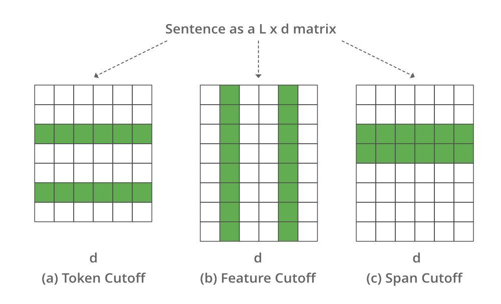
Image representing different cutoffs

To compare the distribution of predictions from different augmentation, we use an additional KL-divergence loss during training.

Dropout:

In 2021, the researchers from the Stanford NLP group propose SimCSE. In the unsupervised scenario, it learns to predict the sentence itself using the DropOut noise In other words, they treat dropout as data augmentation for text sequences.

In the above approach, we take a collection of sentences {[x_i ]}_{i=1}^{m} and treat positive pair as itself x_i^{+} = x_i. During training of Transformers, there is a dropout mask and attention probabilities applied on fully-connected layers. It simply feed the same input to the encoder twice by applying different dropout masks z, z₀ and therefore the training objective function can be defined as:

$l_i =-log \frac{e^{sim(h_i^{z_i},h_i^{z_i^{'}})/ \tau} }{\sum_{j=1}^{N} e^{sim(h_i^{z_i},h_j^{z_j^{'}})/ \tau} }$

where, h_i^{z_i} = f_\theta (x_i, z) is the output and z is the standard mask for dropout.

In supervised setting, we try to leverage the Natural Language Inference dataset (NLI) to predict whether there is entailment (positive pairs) or contradiction (negative pairs) between a given pair of sentences. We extend the $(x_i, x_i^{+}) \, to \, (x_i, x_i^{+}, x_i^{-})$ The objective can be defined as:

$l_i = -log \frac{e^{sim(h_i, h_i^{+})/\tau} }{\sum_{j=1}^{N} (e^{sim(h_i, h_j^{+})/\tau} + e^{sim(h_i, h_j^{-})/\tau})}$

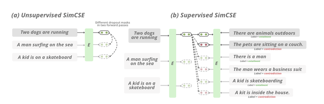
Working of SimCSE

Implementation

In this implementation, we take a few sentences, then applied the SimCSE tokenizer to tokenize the sentence and the model to generate the embedding of inputs, and then we calculate the cosine similarity b/w them.

Python3

# Install PyTorch
! pip install torch==1.7.1+cu110 -f https://download.pytorch.org/whl/torch_stable.html
# clone the repo
!git clone https://github.com/princeton-nlp/SimCSE
# install the requirements
! pip install -r /content/SimCSE/requirements.txt
 
# imports
import torch
from scipy.spatial.distance import cosine
from transformers import AutoModel, AutoTokenizer
 
# Import the pretrained models and tokenizer, this will also download and import th
tokenizer = AutoTokenizer.from_pretrained("princeton-nlp/sup-simcse-bert-base-uncased")
model = AutoModel.from_pretrained("princeton-nlp/sup-simcse-bert-base-uncased")
 
# input sentence
texts = [
    "I am writing an article",
    "Writing an article on Machine learning",
    "I am not writing.",
    "the article on machine learning is already written"
]
 
# tokenize the input
inputs = tokenizer(texts, padding=True, truncation=True, return_tensors="pt")
 
# generate the embeddings
with torch.no_grad():
    embeddings = model(**inputs, output_hidden_states=True, 
                       return_dict=True).pooler_output
# the shape of embedding (# input, 768)
embeddings.shape
 
# print cosine similarity b/w the sentences
for i in range(len(texts)):
  for j in range(len(texts)):
    if (i != j):
      cosine_sim = 1 - cosine(embeddings[i], embeddings[j])
      print("Cosine similarity between \"%s\" and \"%s\" is: %.3f" % (texts[i], texts[j], cosine_sim))

Cosine similarity between “I am writing an article” and “Writing an article on Machine learning” is: 0.515
Cosine similarity between “I am writing an article” and “I am not writing.” is: 0.517
Cosine similarity between “I am writing an article” and “the article on machine learning is already written” is: 0.441
Cosine similarity between “Writing an article on Machine learning” and “I am writing an article” is: 0.515
Cosine similarity between “Writing an article on Machine learning” and “I am not writing.” is: 0.188
Cosine similarity between “Writing an article on Machine learning” and “the article on machine learning is already written” is: 0.807
Cosine similarity between “I am not writing.” and “I am writing an article” is: 0.517
Cosine similarity between “I am not writing.” and “Writing an article on Machine learning” is: 0.188
Cosine similarity between “I am not writing.” and “the article on machine learning is already written” is: 0.141
Cosine similarity between “the article on machine learning is already written” and “I am writing an article” is: 0.441
Cosine similarity between “the article on machine learning is already written” and “Writing an article on Machine learning” is: 0.807
Cosine similarity between “the article on machine learning is already written” and “I am not writing.” is: 0.141

In the above example, we just compare the cosine similarity of the sentences. To know more details about training, please check the training details in the official repository.

References:

Suggest improvement

Understanding Semantic Analysis - NLP

Disentanglement in Beta Variational Autoencoders

Share your thoughts in the comments