Decision Tree Classifiers in R Programming
Last Updated :
23 Dec, 2021
Classification is the task in which objects of several categories are categorized into their respective classes using the properties of classes. A classification model is typically used to,
- Predict the class label for a new unlabeled data object
- Provide a descriptive model explaining what features characterize objects in each class
There are various types of classification techniques such as,
Decision Tree Classifiers in R Programming
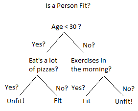
A decision tree is a flowchart-like tree structure in which the internal node represents feature(or attribute), the branch represents a decision rule, and each leaf node represents the outcome. A Decision Tree consists of,
- Nodes: Test for the value of a certain attribute.
- Edges/Branch: Represents a decision rule and connect to the next node.
- Leaf nodes: Terminal nodes that represent class labels or class distribution.
And this algorithm can easily be implemented in the R language. Some important points about decision tree classifiers are,
- It is more interpretable
- Automatically handles decision-making
- Bisects the space into smaller spaces
- Prone to overfitting
- Can be trained on a small training set
- Majorly affected by noise
Implementation in R
The Dataset:
A sample population of 400 people shared their age, gender, and salary with a product company, and if they bought the product or not(0 means no, 1 means yes). Download the dataset Advertisement.csv.
R
dataset = read.csv('Advertisement.csv')
head(dataset, 10)
|
Output:
| |
User ID |
Gender |
Age |
EstimatedSalary |
Purchased |
| 0 |
15624510 |
Male |
19 |
19000 |
0 |
| 1 |
15810944 |
Male |
35 |
20000 |
0 |
| 2 |
15668575 |
Female |
26 |
43000 |
0 |
| 3 |
15603246 |
Female |
27 |
57000 |
0 |
| 4 |
15804002 |
Male |
19 |
76000 |
0 |
| 5 |
15728773 |
Male |
27 |
58000 |
0 |
| 6 |
15598044 |
Female |
27 |
84000 |
0 |
| 7 |
15694829 |
Female |
32 |
150000 |
1 |
| 8 |
15600575 |
Male |
25 |
33000 |
0 |
| 9 |
15727311 |
Female |
35 |
65000 |
0 |
Train the data
To train the data we will split the dataset into a test set and then make Decision Tree Classifiers with rpart package.
R
dataset$Purchased = factor(dataset$Purchased,
levels = c(0, 1))
library(caTools)
set.seed(123)
split = sample.split(dataset$Purchased,
SplitRatio = 0.75)
training_set = subset(dataset, split == TRUE)
test_set = subset(dataset, split == FALSE)
training_set[-3] = scale(training_set[-3])
test_set[-3] = scale(test_set[-3])
library(rpart)
classifier = rpart(formula = Purchased ~ .,
data = training_set)
y_pred = predict(classifier,
newdata = test_set[-3],
type = 'class')
cm = table(test_set[, 3], y_pred)
|
- The training set contains 300 entries.
- The test set contains 100 entries.
Confusion Matrix:
[[62,  6],
 [ 3, 29]]
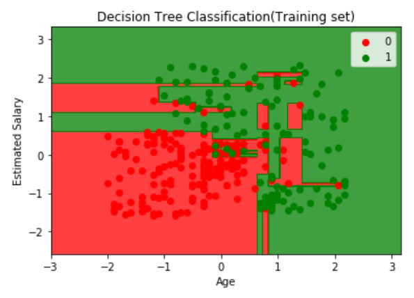
Visualizing the Train Data:
R
library(ElemStatLearn)
set = training_set
X1 = seq(min(set[, 1]) - 1,
max(set[, 1]) + 1,
by = 0.01)
X2 = seq(min(set[, 2]) - 1,
max(set[, 2]) + 1,
by = 0.01)
grid_set = expand.grid(X1, X2)
colnames(grid_set) = c('Age',
'EstimatedSalary')
y_grid = predict(classifier,
newdata = grid_set,
type = 'class')
plot(set[, -3],
main = 'Decision Tree
Classification (Training set)',
xlab = 'Age', ylab = 'Estimated Salary',
xlim = range(X1), ylim = range(X2))
contour(X1, X2, matrix(as.numeric(y_grid),
length(X1),
length(X2)),
add = TRUE)
points(grid_set, pch = '.',
col = ifelse(y_grid == 1,
'springgreen3',
'tomato'))
points(set, pch = 21, bg = ifelse(set[, 3] == 1,
'green4',
'red3'))
|
Output:
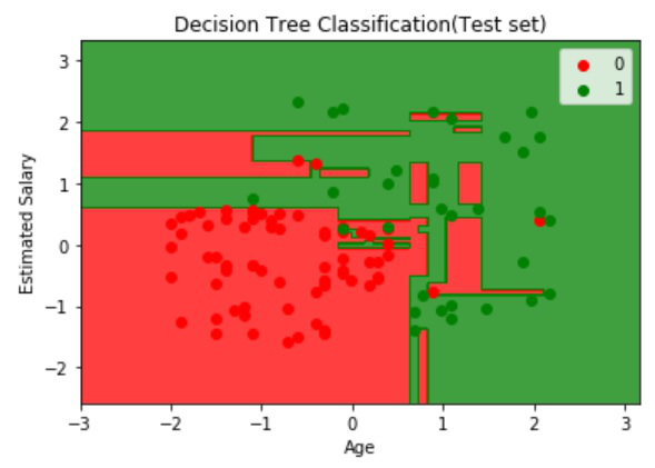
Visualizing the Test Data:
R
library(ElemStatLearn)
set = test_set
X1 = seq(min(set[, 1]) - 1,
max(set[, 1]) + 1,
by = 0.01)
X2 = seq(min(set[, 2]) - 1,
max(set[, 2]) + 1,
by = 0.01)
grid_set = expand.grid(X1, X2)
colnames(grid_set) = c('Age',
'EstimatedSalary')
y_grid = predict(classifier,
newdata = grid_set,
type = 'class')
plot(set[, -3], main = 'Decision Tree
Classification (Test set)',
xlab = 'Age', ylab = 'Estimated Salary',
xlim = range(X1), ylim = range(X2))
contour(X1, X2, matrix(as.numeric(y_grid),
length(X1),
length(X2)),
add = TRUE)
points(grid_set, pch = '.',
col = ifelse(y_grid == 1,
'springgreen3',
'tomato'))
points(set, pch = 21, bg = ifelse(set[, 3] == 1,
'green4',
'red3'))
|
Output:
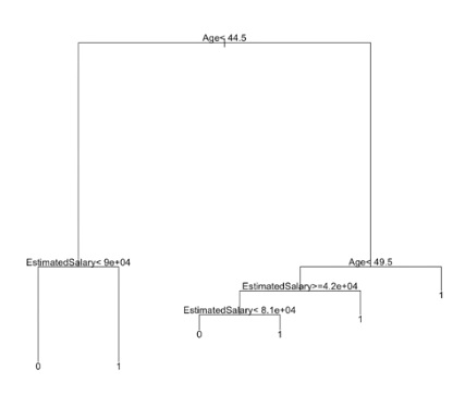
Decision Tree Diagram:
R
plot(classifier)
text(classifier)
|
Output:
Like Article
Suggest improvement
Share your thoughts in the comments
Please Login to comment...