Deep Neural net with forward and back propagation from scratch – Python

Last Updated : 08 Jun, 2020

This article aims to implement a deep neural network from scratch. We will implement a deep neural network containing a hidden layer with four units and one output layer. The implementation will go from very scratch and the following steps will be implemented. Algorithm:

1. Visualizing the input data
2. Deciding the shapes of Weight and bias matrix
3. Initializing matrix, function to be used
4. Implementing the forward propagation method
5. Implementing the cost calculation
6. Backpropagation and optimizing
7. prediction and visualizing the output

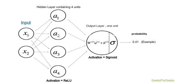
Architecture of the model: The architecture of the model has been defined by the following figure where the hidden layer uses the Hyperbolic Tangent as the activation function while the output layer, being the classification problem uses the sigmoid function.

Model Architecture

Weights and bias: The weights and the bias that is going to be used for both the layers have to be declared initially and also among them the weights will be declared randomly in order to avoid the same output of all units, while the bias will be initialized to zero. The calculation will be done from the scratch itself and according to the rules given below where W1, W2 and b1, b2 are the weights and bias of first and second layer respectively. Here A stands for the activation of a particular layer. $\begin{array}{c} z^{[1]}=W^{[1]} x+b^{[1]} \\ a^{[1](i)}=\tanh \left(z^{[1]}\right) \\ z^{[2]}=W^{[2]} a^{[1]}+b^{[2]} \\ \hat{y}=a^{[2]}=\sigma\left(z^{[2]}\right) \\ y_{\text {prediction}}=\left\{\begin{array}{ll} 1 & \text { if } a^{[2]}>0.5 \\ 0 & \text { otherwise } \end{array}\right. \end{array}$ Cost Function: The cost function of the above model will pertain to the cost function used with logistic regression. 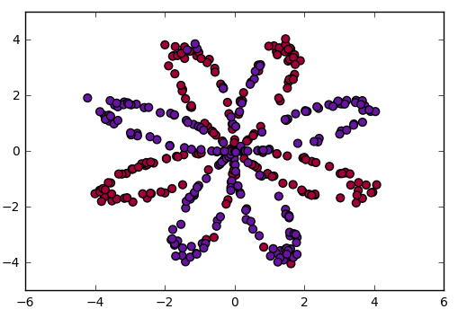Hence, in this tutorial we will be using the cost function: $L = Y * \log \left(Y_{-} p r e d\right)+(1-Y) * \log \left(1-Y_{-} p r e d\right)$ Code: Visualizing the data

# Package imports 
import numpy as np 
import matplotlib.pyplot as plt 
# here planar_utils.py can be found on its github repo 
from planar_utils import plot_decision_boundary, sigmoid, load_planar_dataset 
# Loading the Sample data 
X, Y = load_planar_dataset() 
  
# Visualize the data: 
plt.scatter(X[0, :], X[1, :], c = Y, s = 40, cmap = plt.cm.Spectral); 

Code: Initializing the Weight and bias matrix Here is the number of hidden units is four, so, the W1 weight matrix will be of shape (4, number of features) and bias matrix will be of shape (4, 1) which after broadcasting will add up to the weight matrix according to the above formula. Same can be applied to the W2.

# X --> input dataset of shape (input size, number of examples) 
# Y --> labels of shape (output size, number of examples) 
  
W1 = np.random.randn(4, X.shape[0]) * 0.01
b1 = np.zeros(shape =(4, 1)) 
  
W2 = np.random.randn(Y.shape[0], 4) * 0.01
b2 = np.zeros(shape =(Y.shape[0], 1)) 

Code: Forward Propagation : Now we will perform the forward propagation using the W1, W2 and the bias b1, b2. In this step the corresponding outputs are calculated in the function defined as forward_prop.

def forward_prop(X, W1, W2, b1, b2): 
  
    Z1 = np.dot(W1, X) + b1 
    A1 = np.tanh(Z1) 
    Z2 = np.dot(W2, A1) + b2 
    A2 = sigmoid(Z2) 
      
    # here the cache is the data of previous iteration 
    # This will be used for backpropagation 
    cache = {"Z1": Z1, 
             "A1": A1, 
             "Z2": Z2, 
             "A2": A2} 
      
    return A2, cache 

Code: Defining the cost function :

# Here Y is actual output 
def compute_cost(A2, Y): 
    m = Y.shape[1] 
    # implementing the above formula 
    cost_sum = np.multiply(np.log(A2), Y) + np.multiply((1 - Y), np.log(1 - A2)) 
    cost = - np.sum(logprobs) / m 
      
    # Squeezing to avoid unnecessary dimensions 
    cost = np.squeeze(cost) 
    return cost 

Code: Finally back-propagating function: This is a very crucial step as it involves a lot of linear algebra for implementation of backpropagation of the deep neural nets. The Formulas for finding the derivatives can be derived with some mathematical concept of linear algebra, which we are not going to derive here. Just keep in mind that dZ, dW, db are the derivatives of the Cost function w.r.t Weighted sum, Weights, Bias of the layers.

def back_propagate(W1, b1, W2, b2, cache): 
   
    # Retrieve also A1 and A2 from dictionary "cache" 
    A1 = cache['A1'] 
    A2 = cache['A2'] 
  
    # Backward propagation: calculate dW1, db1, dW2, db2.  
    dZ2 = A2 - Y 
    dW2 = (1 / m) * np.dot(dZ2, A1.T) 
    db2 = (1 / m) * np.sum(dZ2, axis = 1, keepdims = True) 
  
    dZ1 = np.multiply(np.dot(W2.T, dZ2), 1 - np.power(A1, 2)) 
    dW1 = (1 / m) * np.dot(dZ1, X.T) 
    db1 = (1 / m) * np.sum(dZ1, axis = 1, keepdims = True) 
      
    # Updating the parameters according to algorithm 
    W1 = W1 - learning_rate * dW1 
    b1 = b1 - learning_rate * db1 
    W2 = W2 - learning_rate * dW2 
    b2 = b2 - learning_rate * db2 
  
    return W1, W2, b1, b2 

Code: Training the custom model Now we will train the model using the functions defined above, the epochs can be put as per the convenience and power of the processing unit.

# Please note that the weights and bias are global  
# Here num_iteration is epochs 
for i in range(0, num_iterations): 
    
        # Forward propagation. Inputs: "X, parameters". return: "A2, cache". 
        A2, cache = forward_propagation(X, W1, W2, b1, b2) 
          
        # Cost function. Inputs: "A2, Y". Outputs: "cost". 
        cost = compute_cost(A2, Y) 
   
        # Backpropagation. Inputs: "parameters, cache, X, Y". Outputs: "grads". 
        W1, W2, b1, b2 = backward_propagation(W1, b1, W2, b2, cache) 
          
        # Print the cost every 1000 iterations 
        if print_cost and i % 1000 == 0: 
            print ("Cost after iteration % i: % f" % (i, cost)) 

Output with learnt params After training the model, take the weights and predict the outcomes using the forward_propagate function above then use the values to plot the figure of output. You will have similar output.

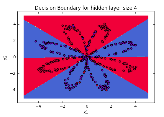
Visualizing the boundaries of data

Conclusion: Deep Learning is a world in which the thrones are captured by the ones who get to the basics, so, try to develop the basics so strong that afterwards, you may be the developer of a new architecture of models which may revolutionalize the community.

Suggest improvement

Multi-Layer Perceptron Learning in Tensorflow

Understanding Multi-Layer Feed Forward Networks

Share your thoughts in the comments

Introduction to Deep Learning

Basic Neural Network

Activation Functions

Artificial Neural Network

Classification

Regression

Hyperparameter tuning

Introduction to Convolution Neural Network

Recurrent Neural Network

Gated Recurrent Unit Networks

Generative Learning

Generative adversarial networks

Reinforcement Learning

Q-Learning in Python

Deep Q Learning