Digital Image Processing Algorithms using MATLAB
Last Updated :
23 Feb, 2021
Like it is said, “One picture is worth more than ten thousand words “A digital image is composed of thousands and thousands of pixels.
An image could also be defined as a two-dimensional function, f(x, y), where x and y are spatial (plane) coordinates and therefore the amplitude of f at any pair of coordinates (x, y) is named the intensity or grey level of the image at that time. When x, y, and therefore the amplitude values of f are all finite, discrete quantities, we call the image a digital image.
Image segmentation using various techniques
1. Basic Filters (masks):
Following filters are used for Edge Detection and discontinuities of an image.
First derivative Operators:
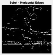
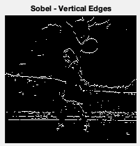
- Sobel Mask– It is also used to detect two kinds of edges in an image one in Vertical and the other in Horizontal direction.
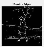
- Prewitt Mask– It is also used to detect two types of edges in an image, Horizontal and Vertical Edges. Edges are calculated by using the difference between corresponding pixel intensities of an image.
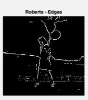
- Robert Mask– It is used in edge detection by approximating the gradient of an image through discrete differentiation.
Second derivative Operators:
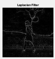
- Laplacian– It is used to find areas of rapid change (edges) in images.
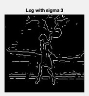
- LOG (Laplacian of a Gaussian) Mask (σ=3)- Since derivative filters are very sensitive to noise, it is common to smoothen the image (using a Gaussian filter) before applying the Laplacian. This two-step process is called the Laplacian of Gaussian (LoG) operation.
- Canny edge detector– It is a popular edge detection algorithm which is a multi-stage and gives the best results when compared to other algorithms.
The gradient-based method such as Prewitt has the most important drawback of being sensitive to noise. The Canny edge detector is less sensitive to noise but more expensive than Robert, Sobel and Prewitt. However, Canny edge detector performs better than all masks.
Applying Sobel Mask:
Input:
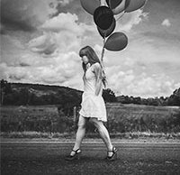
Original Image
Code:
MATLAB
clc;
close all;
clear all;
mycolourimage = imread('image1.jpg');
myimage = rgb2gray(mycolourimage);
subplot(3,3,1);
imshow(myimage); title('Original Image');
sobelhz = edge(myimage,'sobel','horizontal');
subplot(3,3,2);
imshow(sobelhz,[]); title('Sobel - Horizontal Edges');
sobelvrt = edge(myimage,'sobel','vertical');
subplot(3,3,3);
imshow(sobelhz,[]); title('Sobel - Vertical Edges');
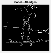
sobelvrthz = edge(myimage,'sobel','both');
subplot(3,3,4);
imshow(sobelvrthz,[]); title('Sobel - All edges');
|
Call the above function using the MATLAB command window.
Output:
Applying Prewitt Mask:
Input:
Original Image
Code:
MATLAB
clc;
close all;
clear all;
mycolourimage = imread('image1.jpg');
myimage = rgb2gray(mycolourimage);
subplot(3,3,1);
imshow(myimage); title('Original Image');
Prewittsedg = edge(myimage,'prewitt');
subplot(3,3,6);
imshow(Prewittsedg,[]); title('Prewitt - Edges');
|
Call the above function using the MATLAB command window.
Output:
Applying Robert Mask:
Input:
Original Image
Code:
MATLAB
clc;
close all;
clear all;
mycolourimage = imread('image1.jpg');
myimage = rgb2gray(mycolourimage);
subplot(3,3,1);
imshow(myimage); title('Original Image');
robertsedg = edge(myimage,'roberts');
subplot(3,3,5);
imshow(robertsedg,[]); title('Roberts - Edges');
|
Call the above function using the MATLAB command window.
Output:
Applying Laplacian Mask:
Input:
Original Image
Code:
MATLAB
clc;
close all;
clear all;
mycolourimage = imread('image1.jpg');
myimage = rgb2gray(mycolourimage);
subplot(3,3,1);
imshow(myimage); title('Original Image');
f=fspecial('laplacian');
lapedg = imfilter(myimage,f,'symmetric');
subplot(3,3,7);
imshow(lapedg,[]); title('Laplacian Filter');
|
Call the above function using the MATLAB command window.
Output:
Applying LOG Mask:
Input:
Original Image
Code:
MATLAB
clc;
close all;
clear all;
mycolourimage = imread('image1.jpg');
myimage = rgb2gray(mycolourimage);
subplot(3,3,1);
imshow(myimage); title('Original Image');
f=fspecial('log',[15,15],3.0);
logedg1 = edge(myimage,'zerocross',[],f);
subplot(3,3,8);
imshow(logedg1); title('Log with sigma 3');
|
Call the above function using the MATLAB command window.
Output:
Applying the Canny edge detector:
Input:
Original Image
Code:
MATLAB
clc;
close all;
clear all;
mycolourimage = imread('image1.jpg');
myimage = rgb2gray(mycolourimage);
subplot(3,3,1);
imshow(myimage); title('Original Image');
cannyedg = edge(myimage,'canny');
subplot(3,3,9);
imshow(cannyedg,[]); title('Canny Edge');
|
Call the above function using the MATLAB command window.
Output:
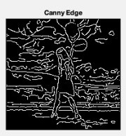
Canny Edge Detector gives the best results compared to other filters/masks used to detect the edges in an image.
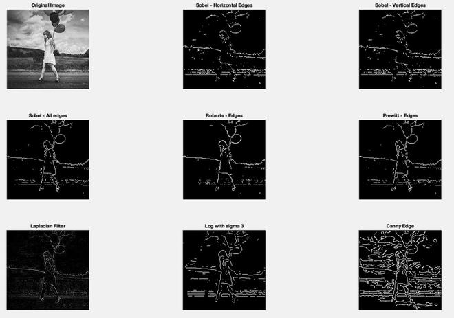
Comparison of all filters used for Edge Detection
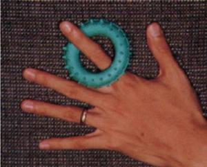
2. Circular Hough Transform:
It is global processing and specialization of Hough Transform. It is used to detect the circles in an input image. This transform is selective to circles and ignores elongated ellipses.
Input:
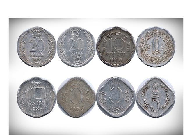
Original Image
Code:
MATLAB
clc;
close all;
clear all;
i=imread('image14.jpg');
imshow(i)
Rmin = 10
Rmax = 50;
[centersDark1, radiiDark1] = imfindcircles(i, [Rmin Rmax],'ObjectPolarity','dark','Sensitivity',0.92);
viscircles(centersDark1, radiiDark1,'LineStyle','--')
|
Call the above function using the MATLAB command window.
Output:
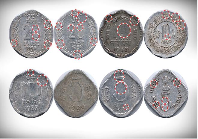
Circular Hough Transformed Image
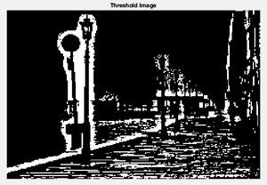
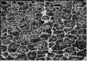
3. Threshold Selection:
It is a local thresholding method in which we are thresholding an input image locally, passing some parameters. We took an image which is already edge operated.
Input:
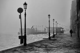
Original Image
Code:
MATLAB
clc;
close all;
clear all;
image = imread('image2.jpeg');
mean_image = imfilter(image, fspecial('average',[15,15]),'replica');
subtract = image - (mean_image+20);
black_white = im2bw(subtract,0);
subplot(1,2,1); imshow(black_white); title('Threshold Image');
subplot(1,2,2); imshow(image); title('Original Image');
|
Call the above function using the MATLAB command window.
Output:
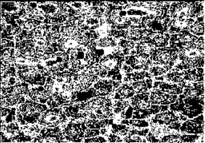
4. Otsu Method:
It is a method of optimum global thresholding. Otsu gives the best result when compared to threshold selection under local thresholding. This method minimizes the weighted within-class variance.
Input:
Original Image
Code:
MATLAB
clc;
close all;
clear all;
I1=imread('image2.jpeg');
imshow(I1);
figure, imhist(I1);
T2 = graythresh(I1);
it2= im2bw(I1,T2);
figure,imshow(it2);
|
Call the above function using the MATLAB command window.
Output:
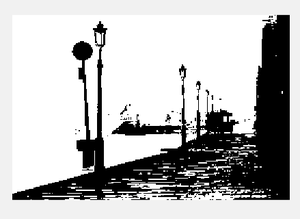
Global Threshold Image
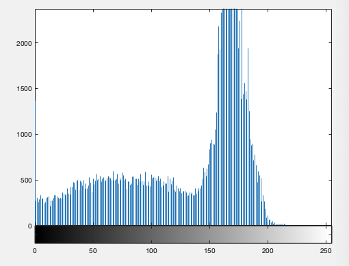
Image Histogram
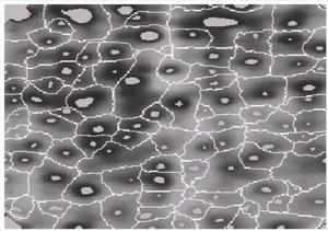
5. Morphological watershed:
In this, the local minima of grey levels give the catchment basins and the local maxima define the watershed lines. In the output image, it is easy to detect the markers.
Input:
Original Image
Code:
MATLAB
clc;
close all;
clear all;
I= imread('image10.png');
I1 = imtophat(I, strel('disk', 10));
figure, imshow(I1);
I2 = imadjust(I1);
figure,imshow(I2);
level = graythresh(I2);
BW = im2bw(I2,level);
figure,imshow(BW);
C=~BW;
figure,imshow(C);
D = ~bwdist(C);
D(C) = -Inf;
L = watershed(D);
Wi=label2rgb(L,'hot','w');
figure,imshow(Wi);
im=I;
|
Call the above function using the MATLAB command window.
Output:

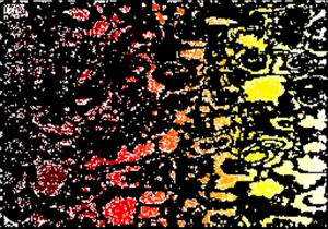
6. K-means Clustering:
It is an algorithm which is used to segment the interest area from the background. Partition the data points into K clusters randomly. Find the centroids of each cluster.
It operates on a 2D array where pixels in rows and RGB in columns. We take mean values for each class (K=3).
Input:
Original Image
Code:
MATLAB
clc;
close all;
clear all;
im = imread('image12.png');
imflat = double(reshape(im, size(im,1) * size(im,2), 3));
K = 3
[kIDs, kC] = kmeans(imflat, K, 'Display', 'iter', 'MaxIter', 150, 'Start', 'sample');
colormap = kC / 256;
imout = reshape(uint8(kIDs), size(im,1), size(im,2));
imwrite(imout - 1, colormap, 'image6.jpg');
|
Call the above function using the MATLAB command window.
Output:
K =
    3
 iter  phase      num          sum
    1      1   178888  1.52491e+08
    2      1     7657  1.45223e+08
    3      1     4597  1.42317e+08
    4      1     3750  1.40017e+08
    5      1     3034  1.38203e+08
    6      1     2187  1.37096e+08
    7      1     1552  1.36481e+08
    8      1     1044  1.36165e+08
    9      1      701  1.36014e+08
   10      1      479  1.35939e+08
   11      1      311  1.35906e+08
   12      1      282  1.35883e+08
   13      1      193   1.3587e+08
   14      1      124  1.35865e+08
   15      1       85  1.35863e+08
   16      1       60  1.35861e+08
   17      1       80   1.3586e+08
   18      1       79  1.35858e+08
   19      1       23  1.35858e+08
   20      1       48  1.35858e+08
   21      1        7  1.35858e+08
Best total sum of distances = 1.35858e+08
Like Article
Suggest improvement
Share your thoughts in the comments
Please Login to comment...