Dual Support Vector Machine

Last Updated : 23 Jan, 2023

Pre-requisite: Separating Hyperplanes in SVM

The Lagrange multiplier equation for the support vector machine. The equation of that can be given by:

$\underset{\vec{w},b}{min} \underset{\vec{a}\geq 0}{max} \frac{1}{2}\left \| w \right \|^{2} - \sum_{j}a_j\left [ \left ( \vec{w} \cdot \vec{x}_{j} \right )y_j - 1 \right ]$

Now, according to the duality principle, the above optimization problem can be viewed as both primal (minimizing over w and b) or dual (maximizing over a).

$\underset{\vec{a}\geq 0}{max}\underset{\vec{w},b}{min} \frac{1}{2}\left \| w \right \|^{2} - \sum_{j}a_j\left [ \left ( \vec{w} \cdot \vec{x}_{j} \right )y_j - 1 \right ]$

Slater condition for convex optimization guarantees that these two are equal problems.

To obtain minimum wrt w and b, the first-order partial derivative wrt these variables must be 0:

$\frac{\partial L}{\partial w} = w -\sum_j a_j y_j x_j =0 \\ w = \sum_j a_j y_j x_j \\ \\ \\ Wrt \, b \\ \\ \frac{\partial L}{\partial b} = -\sum_j a_j y_j =0 \\ \\ \sum_j a_j y_j =0$

Now, put the above equation in the Lagrange multiplier equation and simplify it.

$L = \frac{1}{2}\left ( \sum_i \alpha_i y_i x_i \right )\cdot\left ( \sum_j \alpha_j y_j x_j \right ) - \left ( \sum_i \alpha_i y_i x_i \right )\cdot\left ( \sum_j \alpha_j y_j x_j \right ) - \sum_i\left ( \alpha_i y_i b \right ) + \sum_i\left ( \alpha_{i} \right ) \\$

In the above equation, the term

$\sum_i\left ( \alpha_i y_i b \right ) = 0$ because, b is just a constant and the rest is from the above equation”

$L = \sum \alpha_i - \frac{1}{2}\sum_i \sum_j \alpha_{i} \alpha_{j} y_i y_j \left ( x_i \cdot x_j \right ) \alpha_j \geq 0 \forall j$

To find b, we can also use the above equation and constraint

$\alpha_j > 0 \,for \,some\, j$ :

$y_j\left ( \vec{w}\cdot\vec{x} + b \right ) = 1 \\ \\ y_jy_j\left ( \vec{w}\cdot\vec{x} + b \right ) = y_j \\ \\ y_j \in \left \{ -1,1 \right \} \\ \\ \left ( \vec{w}\cdot\vec{x} + b \right ) = y_j \\ \\ b = y_k - w \cdot x_k \forall k where \, \alpha_k > 0$

Now, the decision rule can be given by:

$y_i = sign(\sum \alpha_{i} y_i \left ( \vec{x}_i \cdot \vec{x} \right ) +b )$

Notice, we can observe from the above rule that the Lagrange multiplier just depends upon the dot product of x_iwith unknown variable x. This dot product is defined as the kernel function, and it is represented by K

$L = \sum \alpha_i - \frac{1}{2}\sum_i \sum_j \alpha_{i} \alpha_{j} y_i y_j K(x_i,x_j) \\ \\ where K = (x_i.x_j)$

Now, for the linearly inseparable case, the dual equation becomes:

$\underset{\alpha}{max} \sum_i \alpha_i - \sum_{i,j} \alpha_i \alpha_j y_i y_j x_i \cdot x_j \\ \\ for, \\ \\ \sum_i \alpha_i y_i =0 \\ \\ 0 \leq \alpha_i \leq C$

Here, we added a constant C, it is required because of the following reasons:

It prevents the value of $\alpha$ from $\alpha \to \infty$ .
It also prevents the models from overfitting, meaning that some misclassification can be accepted.

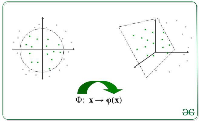
Image depicting transformation

we apply transformation into another space such that the following. Note, we don’t need to specifically calculate the transformation function, we just need to find the dot product of those to get kernel function, however, this transformation function can be easily established.

$K = \phi(i) \cdot \phi(j)$

where,

$\phi()$ is the transformation function.

The intuition behind that many of time a data can be separated by a hyperplane in a higher dimension. Let’s look at this in more detail:

Suppose we have a dataset that contains only 1 independent and 1 dependent variable. The plot below represents the data:

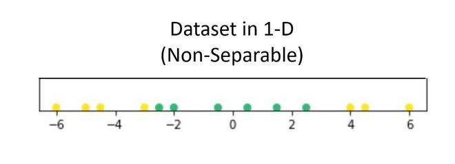
Now, in the above plot, it is difficult to separate a 1D-hyperplane (point) that clearly separates the data points of different classes. But when this transformed to 2d by using some transformation, it provides options for separating the classes.

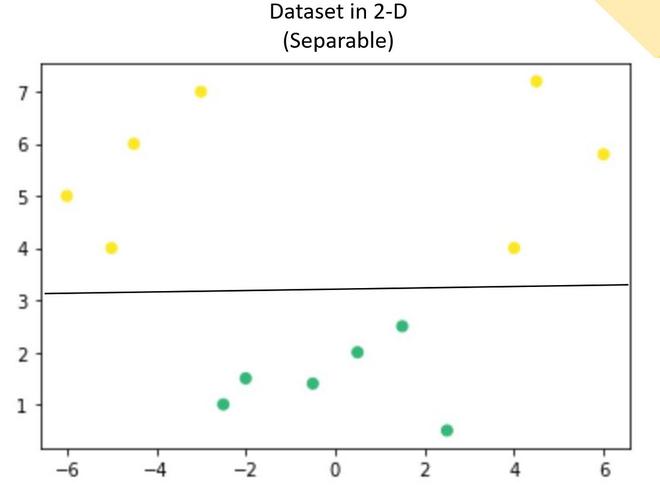
In the above example, we can see that an SVM line can clearly separate the two classes of the dataset.

There is some famous kernel that is used quite commonly:

Polynomials with degree =n

$K(u,v) = (u \cdot v)^{n}$

Polynomials with degree up to n

$K(u,v) = (u \cdot v + 1)^{n}$

Gaussian/ RBF kernel

$K(\vec{u}, \vec{v}) = e^{-\frac{\left \| \vec{u}-\vec{v} \right \|_{2}^{2}}{2 \sigma^2}}$

Implementation

Python3

# code
import numpy as np
import matplotlib.pyplot as plt
from sklearn import svm, datasets
 
# import some data
cancer = datasets.load_breast_cancer()
X = cancer.data[:,:2]
Y = cancer.target
 
X.shape, Y.shape
 
# perform svm with different kernel, here c is the regularizer
h = .02
C=100
lin_svc = svm.LinearSVC(C=C)
svc = svm.SVC(kernel='linear', C=C)
rbf_svc = svm.SVC(kernel='rbf', gamma=0.7, C=C)
poly_svc = svm.SVC(kernel='poly', degree=3, C=C)
 
# Fit the training dataset.
lin_svc.fit(X, Y)
svc.fit(X, Y)
rbf_svc.fit(X, Y)
poly_svc.fit(X, Y)
 
# plot the results
x_min, x_max = X[:, 0].min() - 1, X[:, 0].max() + 1
y_min, y_max = X[:, 1].min() - 1, X[:, 1].max() + 1
xx, yy = np.meshgrid(np.arange(x_min, x_max, h),np.arange(y_min, y_max, h))
 
titles = ['linear kernel',
          'LinearSVC (linear kernel)',
          'RBF kernel',
          'polynomial (degree 3) kernel']
 
plt.figure(figsize=(10,10))
 
for i, clf in enumerate((svc, lin_svc,rbf_svc, poly_svc )):
    # Plot the decision boundary using the above meshgrid we generated
    plt.subplot(2, 2, i + 1)
    Z = clf.predict(np.c_[xx.ravel(), yy.ravel()])
 
    # Put the result into a color plot
    Z = Z.reshape(xx.shape)
    plt.set_cmap(plt.cm.flag_r)
    plt.contourf(xx, yy, Z)
 
    # Plot also the training points
    plt.scatter(X[:, 0], X[:, 1], c=Y)
 
    plt.title(titles[i])
 
plt.show()

((569, 2), (569,))

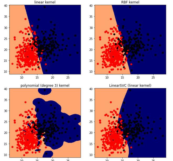
SVM using different kernels.

A Dual Support Vector Machine (DSVM) is a type of machine learning algorithm that is used for classification problems. It is a variation of the standard Support Vector Machine (SVM) algorithm that solves the optimization problem in a different way.

The main idea behind the DSVM is to use a technique called kernel trick which maps the input data into a higher-dimensional space, where it is more easily separable. The algorithm then finds the optimal hyperplane in this higher-dimensional space that maximally separates the different classes.

The dual form of the SVM optimization problem is typically used for large datasets because it is computationally less expensive than the primal form. The primal form of the SVM optimization problem is usually used for small datasets because it gives more interpretable results.

The DSVM algorithm has several advantages over other classification algorithms, such as:

-It is effective in high-dimensional spaces and with complex decision boundaries.
-It is memory efficient, as it only requires a subset of the training data to be used in the decision function.
-It is versatile, as it can be used with various types of kernels, such as linear, polynomial, or radial basis function kernels.

DSVM is mostly used in the fields of bioinformatics, computer vision, natural language processing, and speech recognition. It is also used in the classification of images, text, and audio data.

References:

MIT OCW slides SVM

Suggest improvement

Identifying handwritten digits using Logistic Regression in PyTorch

unicode_literals in Python

Share your thoughts in the comments

Dual Support Vector Machine

Implementation

Python3

References:

Please Login to comment...

Similar Reads

What kind of Experience do you want to share?