GRE Data Analysis | Distribution of Data, Random Variables, and Probability Distributions
Last Updated :
19 Jun, 2019
Distribution of Data:
The distribution of a statistical data set (or a population) is a listing or function showing all the possible values (or intervals) of the data and how often they occur, we can think of a distribution as a function that describes the relationship between observations in a sample space.
Example:
The lifetimes of 800 electric devices were measured. Because the lifetimes had many different values, the measurements were grouped into 50 intervals, or classes, of 10 hours each:
601 to 610 hours, 611 to 620 hours, and so on, up to 1, 091 to 1, 100 hours. The resulting relative frequency distribution, as a histogram, has 50 thin bars and many different bar heights, as shown in Data Analysis Figure below.
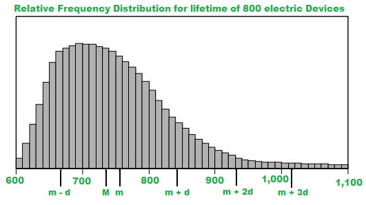 Relative frequency
 is how often something happens divided by all outcomes. As an example here, it can be considered as the number of electric devices having lifetime of (Ex 601 to 610) divided by the total devices.
In the histogram, the
median is represented by M, the
mean is represented by m, and the
standard deviation is represented by d.
- The median, represented by M, is between 730 and 740
- The mean, represented by m, is between 750 and 760
- The sum of areas of all 50 bars of relative frequency is 1
Histograms that represent very large data sets grouped into many classes have a relatively smooth appearance. Consequently, the distribution can be modeled by a smooth curve that is close to the tops of the bars. This curve is called a distribution curve.
The purpose of the distribution curve is to give a good illustration of a large distribution of numerical data that does not depend on specific classes. Property of distribution curve is that the area under the curve in any vertical slice, just like a histogram bar, represents the proportion of the data that lies in the corresponding interval on the horizontal axis.
A random variable can map each value from sample space to a real number and moreover sum of values from real number is always equal to 1
Example:
In an experiment three fair coins are tossed, then sample space is
S = { HHH, HHT, HTH, THH, HTT, TTH, THT, TTT}
Let variable X count the number of times head turns up, hence we call it as Random variable. Moreover random variable is generally represented by X.
Now,
X can take values
3, 2, 1, 0
P(X = 1) is probability of occurring head one time,
P(X = 1) = P(THT) + P(TTH) + P(HTT) = 3/8
Types of random variable:
- Discrete Random Variable:
A variable that can take one value from a discrete set of values.
Example:
Let x denote the sum of dice, Now x is discrete random variable as it can take one value from the set { 2, 3, 4, 5, 6, 7, 8, 9, 10, 11, 12 }, since the sum of two dice can only be one of these values.
- Continuous Random Variable:
A variable that can take one value from a continuous range of values.
Example:
x denotes the volume of water in a 500 ml cup. Now x may be a number from 0 to 500, any of which value, x may take.
Probability Distribution:
Probability distributions indicate the likelihood of an event or outcome.
P(x) = the likelihood that random variable takes a specific value of x.
Example:
In an experiment three fair coins are tossed, then sample space is,
S = {HHH, HHT, HTH, THH, HTT, TTH, THT, TTT}
X is random variable having values 3, 2, 1, 0 then
P(X = 0) = P(TTT) = 1/8
P(X = 1) = P(HTT) + P(TTH) + P(THT) = 3/8
P(X = 2) = P(HHT) + P(HTH) + P(THH) = 3/8
P(X = 3) = P(HHH) = 1/8
Therefore,
| X (random variable) |
P(X) |
| 0 |
1/8 |
| 1 |
3/8 |
| 2 |
3/8 |
| 3 |
1/8 |
This table is called the probability distribution of random variable X.
Distribution can be divided into
2 types:
- Discrete distribution:
Based on discrete random variable, examples are Binomial Distribution, Poisson Distribution.
- Continuous distribution:
Based on continuous random variable, examples are Normal Distribution, Uniform Distribution, Exponential Distribution.
Probability Mass Function:
Let x be discrete random variable then its Probability Mass Function p(x) is defined such that
1. p(x) 0
2.
0
2.  = 1
3. p(x) = P(X=x)
= 1
3. p(x) = P(X=x)
Probability Density Function:
Let x be continuous random variable then probability density function F(x) is defined such that
1. F(x)  0
2.  = 1
3. P(a < x < b) =
= 1
3. P(a < x < b) = 
Properties of Discrete Distribution:
1.  = 1
2. E(x) =
= 1
2. E(x) =  3. V(x) =
Properties of Continuous Distribution:
1.  = 1
2. E(x) =
= 1
2. E(x) =  3. V(x) =
4. p(a < x < b) =
3. V(x) =
4. p(a < x < b) = 
Where,
E(x) denotes expected value or average value of the random variable x,
V(x) denotes the variance of the random variable x.
Types of Distributions:
Like Article
Suggest improvement
Share your thoughts in the comments
Please Login to comment...