How To Create a Tornado Chart In Excel?

Tornado charts are a special type of Bar Charts. They are used for comparing different types of data using horizontal side-by-side bar graphs. They are arranged in decreasing order with the longest graph placed on top. This makes it look like a 2-D tornado and hence the name.

Creating a Tornado Chart in Excel:

Follow the below steps to create a Tornado Chart In Excel:

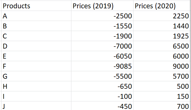
Step 1: Open Excel and Prepare your Data table. Start writing your data in a table with appropriate headers for each column. Once this is done, make sure you select either of the columns and set all of its values to negative i.e., if the original value in Header Xyz is 2000, then change it to negative two thousand or “-2000” as shown below.

 Step 2: Select the entire table using L-Shift and the arrow keys. Then, go to the Data section from the top bar and select “Sort.”

Now, set the “Sort by” value to the Header of your Negative column and set the “Order” as “Largest to Smallest” as shown below, and click OK.

Sorting the data

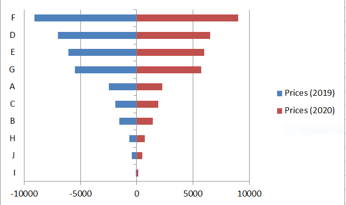
Step 3: Representing the above data in Bar Chart

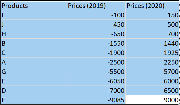
Sorted data

Now, select the entire table. Go to “Insert” and select Bar. Under “Bar”, select the Stacked bar option and wait for your tornado chart to open up.

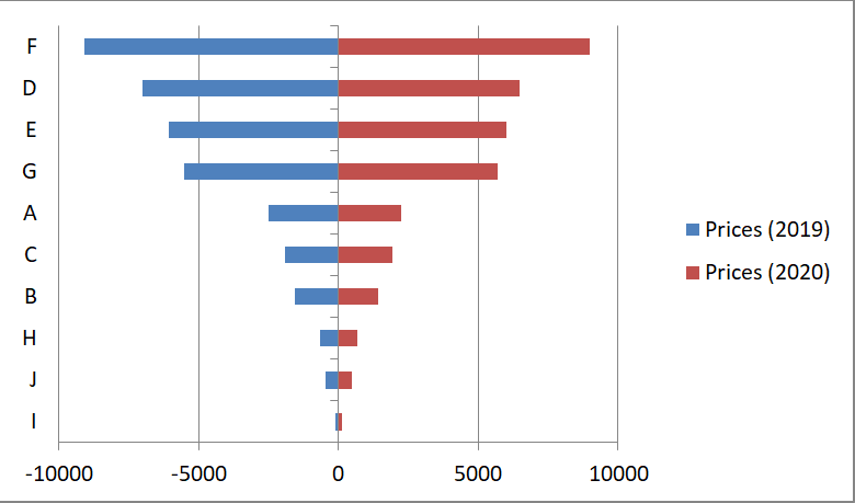
Converting a Tornado Chart to a Butterfly Chart:

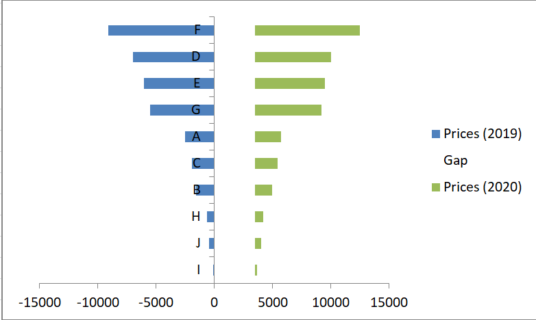
Butterfly Chart

To convert the above Tornado Chart into a Butterfly chart, as shown above, add a third column with constant values and place it between the Negative and the Positive columns.

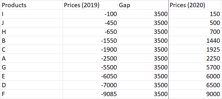
Notice the Gap Column

Now, repeat the process for the Tornado Chart and then select the Gap column and fill it with the color White. The Butterfly chart is ready.

Note: This article has been written based on Microsoft Excel 2010, but all steps are applicable for all later versions