How to Create an Excel Step Chart Formula Using the Small Function?

A step Chart is a kind of line chart which uses horizontal and vertical lines to connect two different data points and forms a step-like structure. Unlike a line chart, it does not use the shortest distance to connect two different data points. A step chart is used to display data that varies unevenly over time. A step chart is useful in representing the inflation rate change, interest rate change, tax rate change, etc.

 

In a step chart, a single step contains horizontal and vertical lines. The horizontal line is used to represent the constancy in the data and the vertical line represents the change in the magnitude of the data.

Steps to Create an Excel Step Chart Formula using Small Function

In this example, we will be using the last 10 years’ change in the inflation rate of India to publish a step chart.

Step 1: Create a Dataset. In this step, we will be creating the dataset using the following inflation data and inserting them in a table as shown below picture.

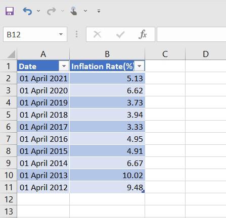
Fig2 – Dataset

Step 2: Inserting Formula. Excel by default doesn’t provide any template for inserting step charts. So, we will use SMALL() and VLOOKUP() functions to create a step chart. First, we will be inserting two more columns for reference as Year and Rate respectively.

 

SMALL() Function

We will be changing the column type for our Year column to Date. After this, we will be using the small function (Here, in cell C3) as given below for our Year column.

=SMALL(Table2[Date],TRUNC(ROW()/2,0))

 

Note: Here, the table name for our Date column is Table2, when you are writing for your example, it may appear different.

This =SMALL(Table2[Date], TRUNC(ROW()/2,0)) will be returning the smallest value. We are truncating the Row and then dividing it by 2 so, that excel will repeat the same value in two consecutive rows.

VLOOKUP() Function

Now, we will be using the following VLOOKUP formula in our Rate column (Here, column-D).

=IF(ISNUMBER(C1),IF(C2<>C1,D1,VLOOKUP(C2,Table2,2,FALSE)),VLOOKUP(C2,Table2,2,FALSE))

Using the above VLOOKUP formula excel will be doing the following calculations:

• Excel checks whether its cursor data is at the start, middle, or end of the dataset.
• If cell C1 contains a number, excel understands its cursor is in the middle or end of the dataset and its cursor will be pushed to the second if-statement. 
• The second if-statement checks whether the excel cursor is in the first or second repeating value, which is created by the SMALL() function in the above steps.
• If C2<>C1, the excel cursor is pointing to the second repeated value and needs to return(repeat) the value of cell D1.
• If C2==C1, the excel cursor is pointing to the first repeated value and needs to VLOOKUP the data in column C.
• The final VLOOKUP() function checks the first if-statement, if it is not a number, then excel will VLOOKUP the value in column C.

Once we have put the small() and the lookup() function in specified cells(Here, C2 and D2) we need to drag it down till the cells get #NUM! For this, we need to hold the rightmost corner of cells C2 and D2 and drag it down.

 

Once we drag down the small() and vlookup() formula we will have the following dataset.

 

Step 3: Inserting Chart. In this step, we will insert a line chart using the Year and Date column (Here, columns C and D). For this Select Data and then go to Insert on the top of the ribbon and then click on Charts and then select Line Chart.

 

Step 4: Output. Once we insert the line chart, we will get the output as a step chart.