Bivariate data is the most used type of data representation for the plotting of scatter plots . The data depends on two variables as its name suggests, and it is analyzed using different machine-learning algorithms, using different charts, etc. Bivariate can be performed using different methods. Among those Linear regression is one of the most used algorithms for bivariate data.
In this article, we will learn how to deal with bivariate data and analyze it using scatter plots.
What is Bivariate Data
Bivariate data is data which have two variable dependencies. The data can be either Quantitative or Qualitative. The value of one variable changes accordingly with the value of the second variable. The Quantitative bivariate data can be represented in the form of a scatter plot, and Qualitative variable data can be represented in the form of a frequency distribution table. A correlation can exist in bivariate data, the correlation value ranges from -1 and 1.
What are Scatter Plots
Scatter plots are graphs that represent the relation between two variables. It is simply said as plotting points, on the X and Y axis. They are very useful for data analysis or regression analysis. The independent attributes are plotted on X-axis, while dependent attributes are plotted on Y-axis.
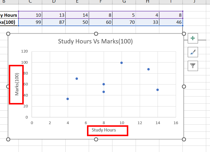
For example, you are given a scatter plot of Study Hours and Marks(100).
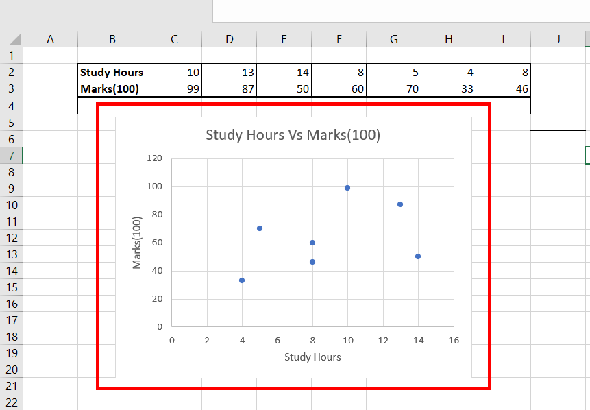
Example: Scatter Plot
What is Linear Regression
Linear Regression is a machine learning model, which is used to predict the future values of a dependent variable, with respect to the best-fit line. The best-fit line is the line that passes through the data points, such that they have the minimum distance error sum from all the points. This is also called a trend line. Excel one-click functionality, to display the equation of the trend line, which is achieved from the machine learning linear regression algorithm.
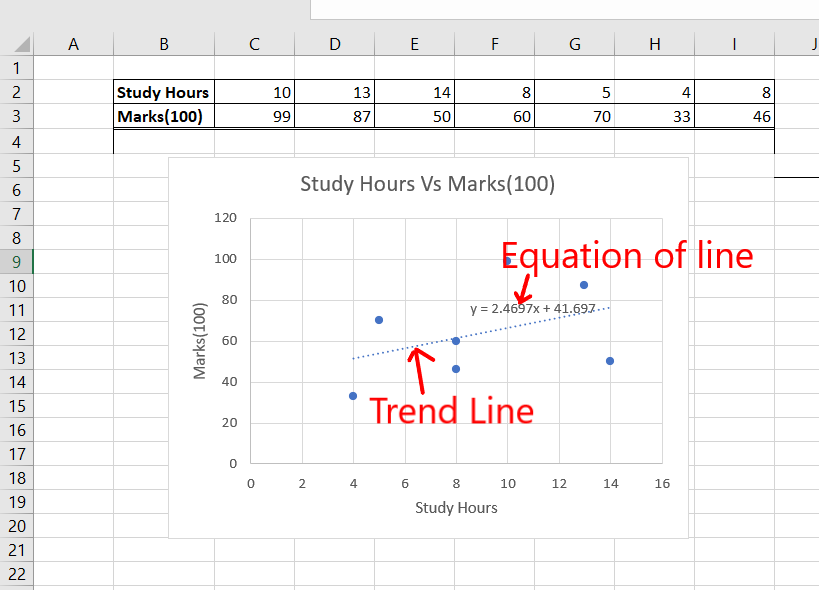
Example : Linear Regression
How to Plot Bivariate Data using Scatter Plot – Steps
Now, we will learn how to create a scatter plot and add a trend line, which will help us analyze the bivariate data in a better way. Lets begin with the help of an example.
For example, Arushi is the class teacher of the tenth (X)th class, she collected data from her students, how many hours they use to study in a day, and added the marks achieved corresponding to that student, her task is to analyze this bivariate data in excel, by plotting it in a scatter plot.
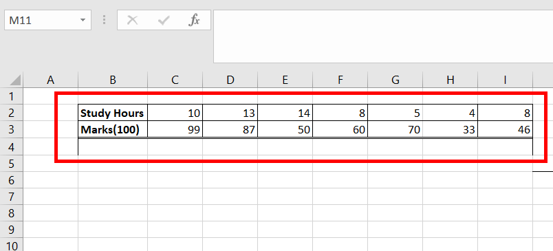
Adding Marks and Study Hours
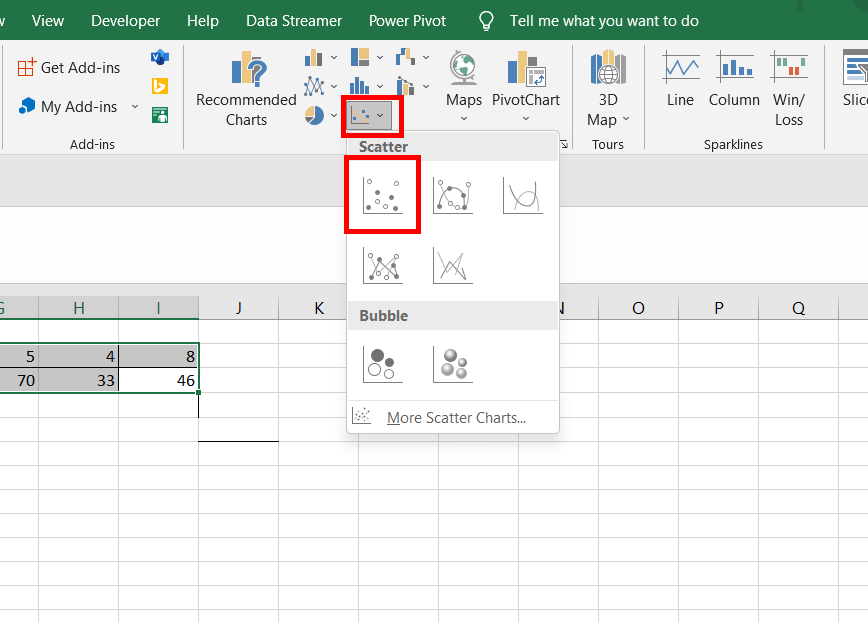
Step 1: Access the Insert Tab
Select the data you entered, and go to the Insert Tab. After selecting Insert Tab you have to add a scatter chart.
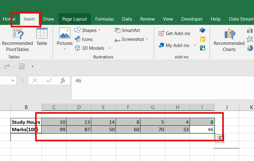
Selecting the Data and Accessing Insert
Step 2: Select the Scatter Chart
Find the Charts section, and under the section go to the scatter chart and select it.
Select Scatter Chart
Step 3: Chart is Successfully Created
As you click on Scatter charts option, a chart is created, between Study Hours (X-axis) and Marks Scored (Y-axis).
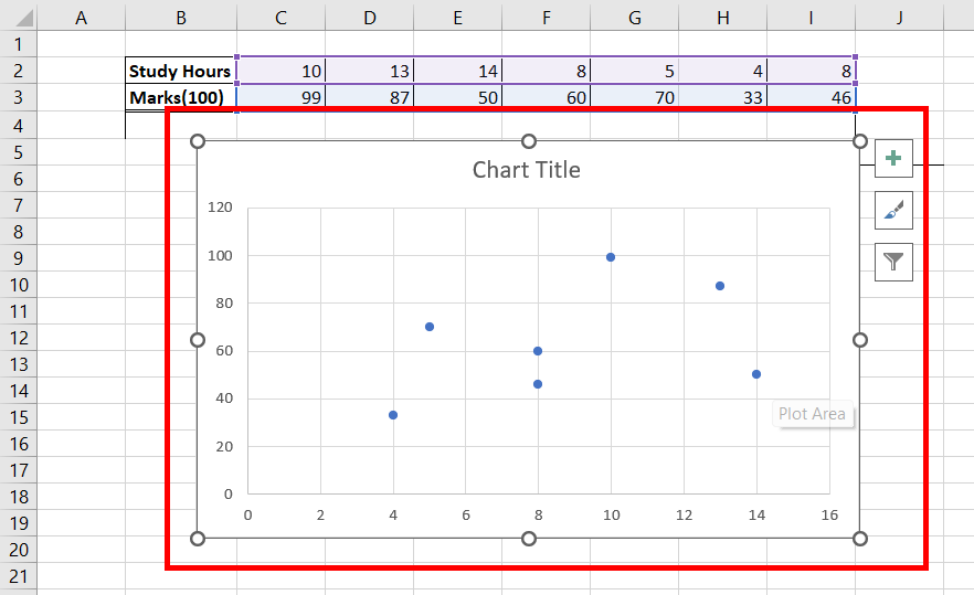
Chart Creatted
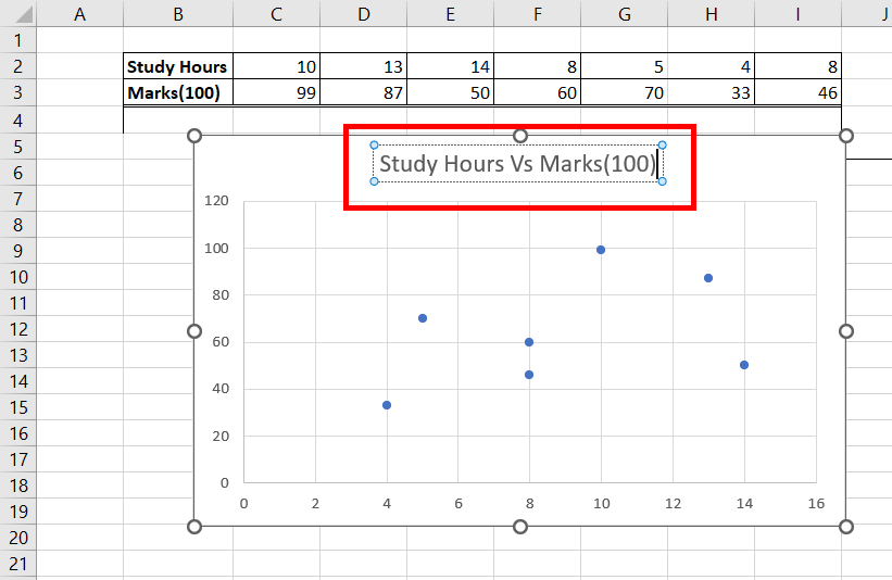
Step 4: Adding Custom Title
Add a custom title to the prepared chart i.e. Study Hours Vs Marks(100) by double clicking on the Tilte Box.
Add Custom Tilte
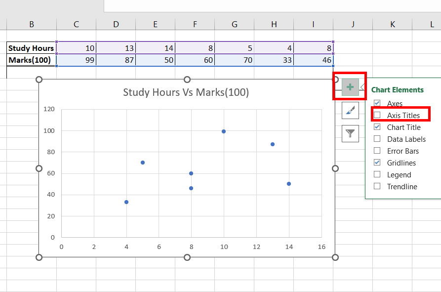
Step 5: Add Titles to X and Y Axis
Select the chart, click on the plus(+) button, and check the box Axis Titles. This adds the name of the X-Axis and Y-Axis.
Select Axis Titles
Step 6: Preview Titles Added to X and Y axis
The Axis titles, box is added, with the default name as Axis Title.

Titles Added
Step 7: Edit the Titles of X and Y Axis
On the X and Y axis, select the Axis Title, and change the name to Study Hours and Marks(100) respectively.
Titles Name Added
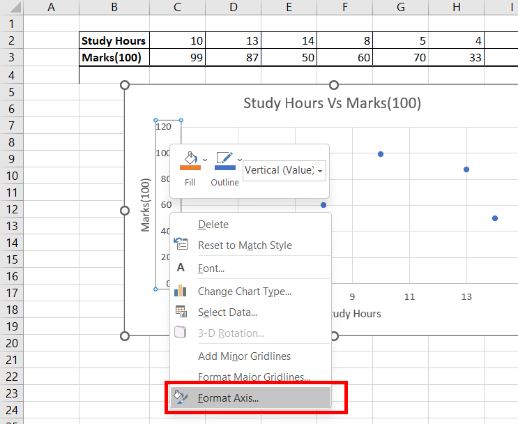
Step 8: Select X Axis
Select the X-Axis chart area, and right-click on it. A drop-down appears, select the format axis.
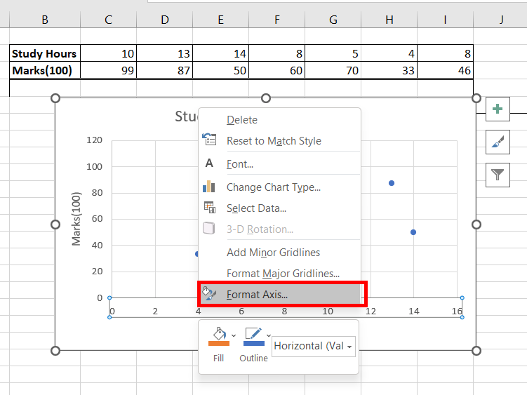
Select X axis
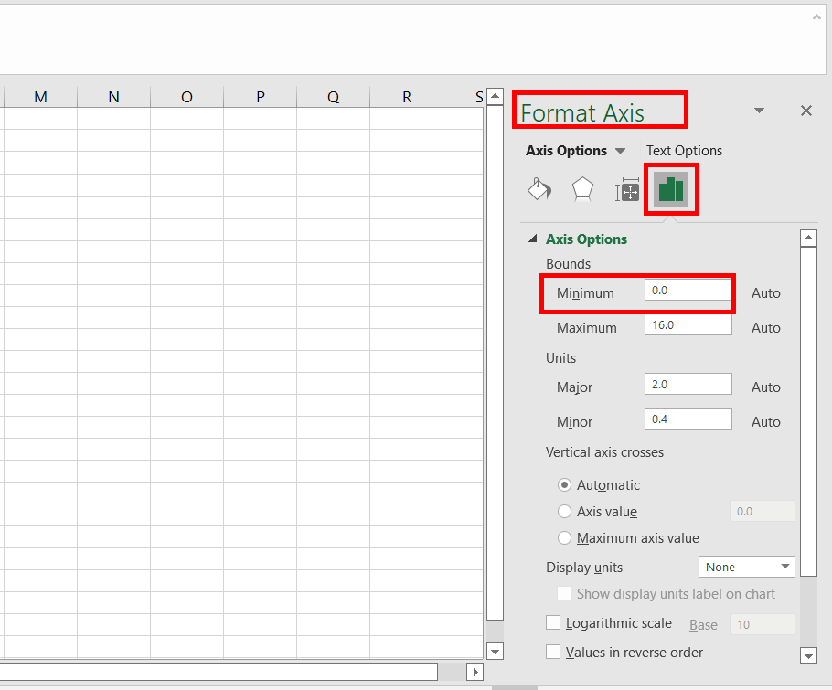
Step 9: Go to Format Axis
A Format Axis, dialogue box appears, at the right-most side of your screen. Under the Axis Options, the default value of minimum is 0. We can see our data starts after value 4. To have better visualization, we could change the minimum value from 0 to 3. This totally depends on the user, one can provide any value as the minimum value.
Go to Format Axis and Check Minimum Value
Step 10: Change Axis Value
Change the minimum value from 0 to 3. Press Enter.

Giving Value according to data
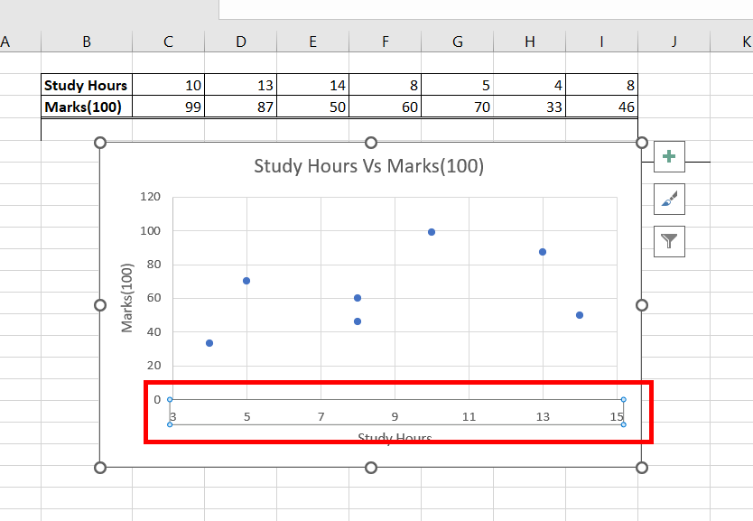
Step 11: Preview Changed X Axis Value
Now, you can observe, our X-axis starts from value 3.
Value Changed
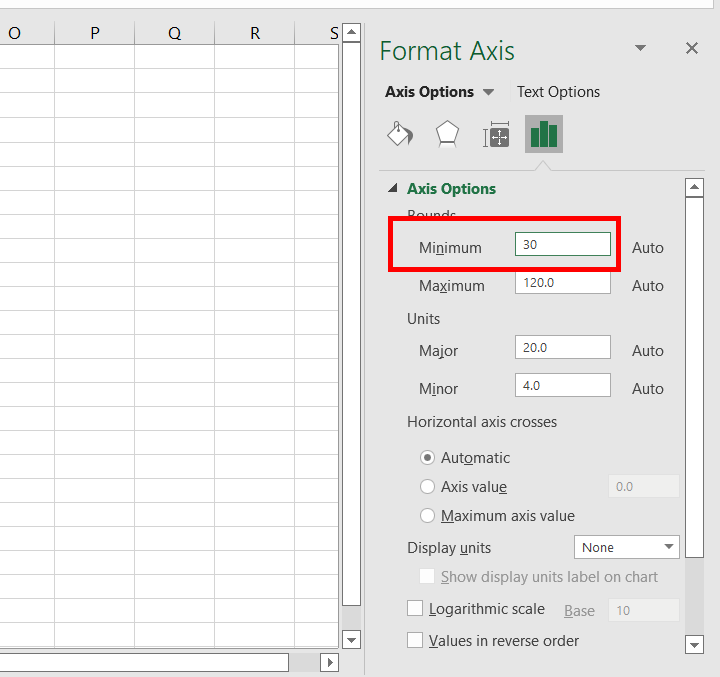
Step 12: Select Format Axis For Y Axis
Repeat the same for Y-axis. Select the Y-axis chart area, and right-click on it. A drop-down appears, select the format axis.
Select Format Axis
Step 13: Check Minimum Value and Change It
A Format Axis, a dialogue box appears, at the right-most side of your screen. Under the Axis Options, the default value of minimum is 0. We can see our data starts after value 40. To have better visualization, we could change the minimum value from 0 to 30. This totally depends on the user, one can provide any value as the minimum value. Press Enter.
Check Minimum Value
Step 14: Preview Changed Value
Now, you observe, our Y-axis starts from value 30.
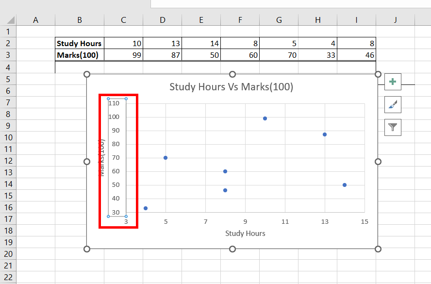
Value Changed
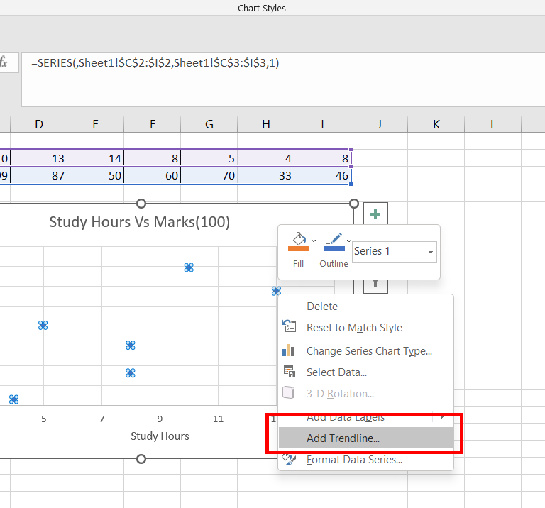
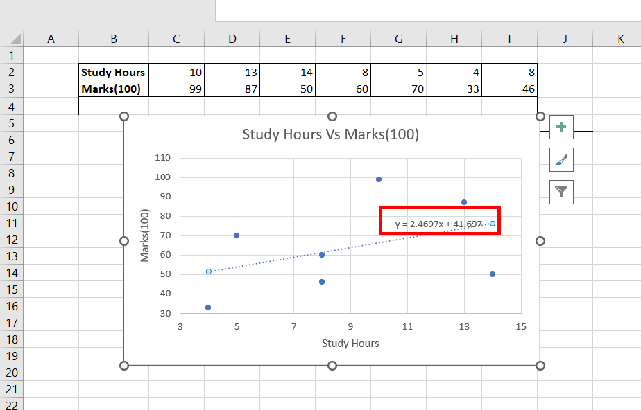
Step 15: Add Trendline
Now, the only work left is to add a trend line, and an equation of the best-fit line, which is part of our linear regression. Select the data points, and right-click on them. Select Add Trendline. This adds the trend line to your chart.
Select Trendline
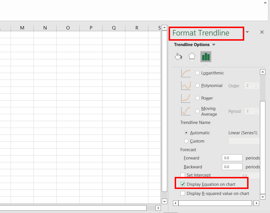
Step 16: Go to Format Trendline and Select Display Eaquation On Chart
Also, a Format Trendline dialogue box appears, at the right-most side of your screen. Under the Trendline Options, check the box, Display equation on the chart.
Select Display on Chart
Step 17: Preview Added Trendline
A Trend line and its equation is added to your chart.
Trend line is added
Step 18: Use CORREL Function
Our Bivariate data is plotted, efficiently for analytical purposes. The only work left is to add the correlation value between the two variables.
Note: Use =CORREL(C2:I2, C3:I3) function, to add a correlation between the variables. Press Enter.

Using CORREL Function
Step 19: Value is Positive
The correlation value is 0.396 i.e. positive, which signifies that as the study hours increase, the marks of students also increase.

Correlation Value is Positive
Conclusion
With the above mentioned steps you can easily plot Bivariate data in Excel using Scatter Plots. This is easy to do. You can easily corelate two variables and find the relationship between them which is very useful in data analysis and understanding. It also looks more presentable and is way organised.
FAQs
What is plotting bivariate data in Excel?
Plotting Bivariate data in Excel means creating a graph that displays the relationship between two different things that are related to each other. The data set you use for this graph consists of pairs of values, where each pair represents a value from one thing and its corresponding value from another thing. By plotting this data, you can visualize patterns, trends, correlations, or associations between the two variables.
How we can create a scatter plot for bivariate data in Excel?
You can follow the below steps to create a Scatter plot in Excel for bivariate data:
Step 1: Enter the data into two columns, one for each variable.
Step 2: Select the data range that includes both columns.
Step 3: Go to the “Insert” tab in the Excel ribbon.
Step 4: Click on the “Scatter” chart type and choose the scatter plot style you prefer.
Can we add a trendline to the scatter plot in Excel?
Yes, you can add a trendline to the Scatter plot in Excel to visualize the general trend or relationship between the variables. To add a trendline follow the below steps:
Step 1: Click on the Scatter plot to select it.
Step 2: Go to the “Chart design” tab in the Excel Ribbon.
Step 3: Click on “Add Chart Element” and choose “Trendline”.
Step 4: Select the type of tradeline you want to add.
Step 5: The trendline will be now added to the scatter plot, and you can format it by right- click and select “Format Trendline”.
How can we create other types of bivariate plots in Excel?
Excel allows us to create other chart types suitable for visualizing bivariate data, including line charts, bubble charts, and 3D Scatter plots. The steps to create these plots are similar to creating a scatter plot. You should arrange your data differently or use specific chart types from the “Insert” tab based on your requirements.
Like Article
Suggest improvement
Share your thoughts in the comments
Please Login to comment...