Implementation of Lasso, Ridge and Elastic Net

Last Updated : 15 May, 2021

In this article, we will look into the implementation of different regularization techniques. First, we will start with multiple linear regression. For that, we require the python3 environment with sci-kit learn and pandas preinstall. We can also use google collaboratory or any other jupyter notebook environment.
First, we need to import some packages into our environment.

Python3

import pandas as pd
import numpy as np
import matplotlib.pyplot as plt
from sklearn import datasets
from sklearn.model_selection import train_test_split
from sklearn.linear_model import LinearRegression

We are going to use the Boston house prediction dataset. This dataset is present in the datasets module of sklearn (scikit-learn) library. We can import this dataset as follows.

Python3

# Loading pre-defined Boston Dataset
boston_dataset = datasets.load_boston()
print(boston_dataset.DESCR)

Output:

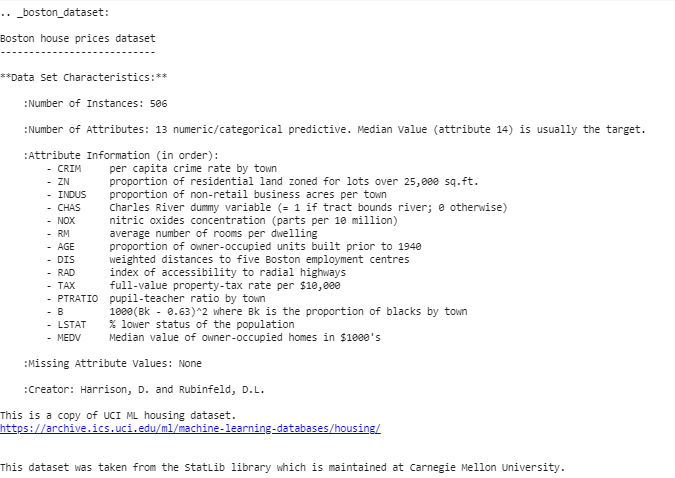
We can conclude from the above description that we have 13 independent variable and one dependent (House price) variable. Now we need to check for a correlation between independent and dependent variable. We can use scatterplot/corrplot for this.

Python3

# Generate scatter plot of independent vs Dependent variable
plt.style.use('ggplot')
fig = plt.figure(figsize = (18, 18))
 
for index, feature_name in enumerate(boston_dataset.feature_names):
    ax = fig.add_subplot(4, 4, index + 1)
    ax.scatter(boston_dataset.data[:, index], boston_dataset.target)
    ax.set_ylabel('House Price', size = 12)
    ax.set_xlabel(feature_name, size = 12)
 
plt.show()

The above code produce scatter plots of different independent variable with target variable as shown below

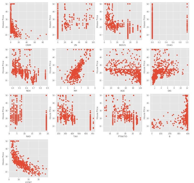
We can observe from the above scatter plots that some of the independent variables are not very much correlated (either positively or negatively) with the target variable. These variables will get their coefficients to be reduced in regularization.
Code : Python code to pre-process the data.

Python3

# Load the dataset into Pandas Dataframe
boston_pd = pd.DataFrame(boston_dataset.data)
boston_pd.columns = boston_dataset.feature_names
boston_pd_target = np.asarray(boston_dataset.target)
boston_pd['House Price'] = pd.Series(boston_pd_target)
 
# input 
X = boston_pd.iloc[:, :-1]
 
#output
Y = boston_pd.iloc[:, -1]
 
print(boston_pd.head())

Now, we apply train-test split to divide the dataset into two parts, one for training and another for testing. We will be using 25% of the data for testing.

Python3

x_train, x_test, y_train, y_test = train_test_split(
    boston_pd.iloc[:, :-1], boston_pd.iloc[:, -1], 
    test_size = 0.25)
 
print("Train data shape of X = % s and Y = % s : "%(
    x_train.shape, y_train.shape))
 
print("Test data shape of X = % s and Y = % s : "%(
    x_test.shape, y_test.shape))

Multiple (Linear) Regression
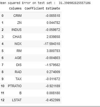
Now it’s the right time to test the models. We will be using multiple Linear Regression first. We train the model on training data and calculate the MSE on test.

Python3

# Apply multiple Linear Regression Model
lreg = LinearRegression()
lreg.fit(x_train, y_train)
 
# Generate Prediction on test set
lreg_y_pred = lreg.predict(x_test)
 
# calculating Mean Squared Error (mse)
mean_squared_error = np.mean((lreg_y_pred - y_test)**2)
print("Mean squared Error on test set : ", mean_squared_error)
 
# Putting together the coefficient and their corresponding variable names 
lreg_coefficient = pd.DataFrame()
lreg_coefficient["Columns"] = x_train.columns
lreg_coefficient['Coefficient Estimate'] = pd.Series(lreg.coef_)
print(lreg_coefficient)

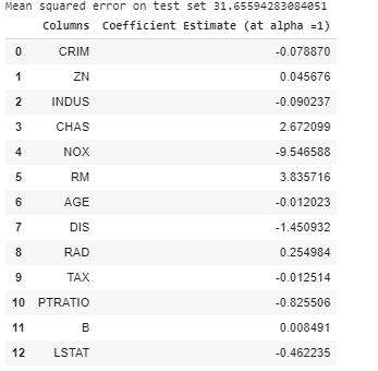
Output:

Let’s plot a bar chart of above coefficients using matplotlib plotting library.

Python3

# plotting the coefficient score
fig, ax = plt.subplots(figsize =(20, 10))
 
color =['tab:gray', 'tab:blue', 'tab:orange', 
'tab:green', 'tab:red', 'tab:purple', 'tab:brown', 
'tab:pink', 'tab:gray', 'tab:olive', 'tab:cyan', 
'tab:orange', 'tab:green', 'tab:blue', 'tab:olive']
 
ax.bar(lreg_coefficient["Columns"], 
lreg_coefficient['Coefficient Estimate'], 
color = color)
 
ax.spines['bottom'].set_position('zero')
 
plt.style.use('ggplot')
plt.show()

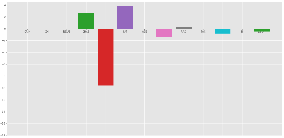
Output:

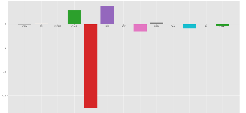
As we can observe that lots of the variables have an insignificant coefficient, these coefficients did not contribute to the model very much and need to regulate or even eliminate some of these variables.

Ridge Regression:
Ridge Regression added a term in ordinary least square error function that regularizes the value of coefficients of variables. This term is the sum of squares of coefficient multiplied by the parameter The motive of adding this term is to penalize the variable corresponding to that coefficient not very much correlated to the target variable. This term is called L₂ regularization.
Code : Python code to use Ridge regression

Python3

# import ridge regression from sklearn library
from sklearn.linear_model import Ridge
 
# Train the model 
ridgeR = Ridge(alpha = 1)
ridgeR.fit(x_train, y_train)
y_pred = ridgeR.predict(x_test)
 
# calculate mean square error
mean_squared_error_ridge = np.mean((y_pred - y_test)**2)
print(mean_squared_error_ridge)
 
# get ridge coefficient and print them
ridge_coefficient = pd.DataFrame()
ridge_coefficient["Columns"]= x_train.columns
ridge_coefficient['Coefficient Estimate'] = pd.Series(ridgeR.coef_)
print(ridge_coefficient)

Output: The value of MSE error and the dataframe with ridge coefficients.

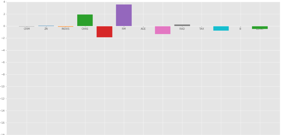
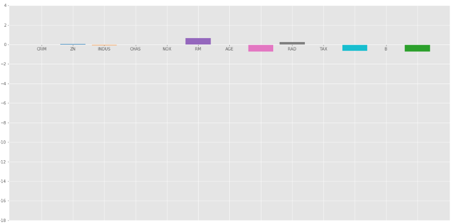
The bar plot of above data is:

Ridge Regression at $\alpha$ =1

In the above graph we take $\alpha$ = 1.
Let’s look at another bar plot with $\alpha$ = 10

Ridge regression at $\alpha$ = 10

As we can observe from the above plots that $\alpha$ helps in regularizing the coefficient and make them converge faster.
Notice that the above graphs can be misleading in a way that it shows some of the coefficients become zero. In Ridge Regularization, the coefficients can never be 0, they are just too small to observe in above plots.

Lasso Regression:
Lasso Regression is similar to Ridge regression except here we add Mean Absolute value of coefficients in place of mean square value. Unlike Ridge Regression, Lasso regression can completely eliminate the variable by reducing its coefficient value to 0. The new term we added to Ordinary Least Square(OLS) is called L₁ Regularization.
Code : Python code implementing the Lasso Regression

Python3

# import Lasso regression from sklearn library
from sklearn.linear_model import Lasso
 
# Train the model
lasso = Lasso(alpha = 1)
lasso.fit(x_train, y_train)
y_pred1 = lasso.predict(x_test)
 
# Calculate Mean Squared Error
mean_squared_error = np.mean((y_pred1 - y_test)**2)
print("Mean squared error on test set", mean_squared_error)
lasso_coeff = pd.DataFrame()
lasso_coeff["Columns"] = x_train.columns
lasso_coeff['Coefficient Estimate'] = pd.Series(lasso.coef_)
 
print(lasso_coeff)

Output: The value of MSE error and the dataframe with Lasso coefficients.

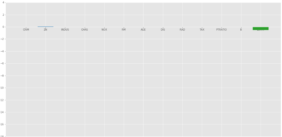
Lasso Regression with $\alpha$ = 1

The bar plot of above coefficients:

Lasso Regression with $\alpha$ =1

The Lasso Regression gave same result that ridge regression gave, when we increase the value of $\alpha$ . Let’s look at another plot at $\alpha$ = 10.

Elastic Net :
In elastic Net Regularization we added the both terms of L₁ and L₂ to get the final loss function. This leads us to reduce the following loss function:
$L_{elastic-Net}\left ( \hat\beta \right )= \left ( \sum \left ( y - x_i^J\hat{\beta} \right )^2 \right )/2n+\lambda \left ( (1 -\alpha )/2 * \sum_{j=1}^{m} \hat{\beta_{j}^{2}}+\alpha * \sum_{j=1}^{m} \left \| \hat{\beta_{j}} \right \| \right)$
where $\alpha$ is between 0 and 1. when $\alpha$ = 1, It reduces the penalty term to L₁ penalty and if $\alpha$ = 0, it reduces that term to L₂
penalty.
Code : Python code implementing the Elastic Net

Python3

# import model
from sklearn.linear_model import ElasticNet
 
# Train the model
e_net = ElasticNet(alpha = 1)
e_net.fit(x_train, y_train)
 
# calculate the prediction and mean square error
y_pred_elastic = e_net.predict(x_test)
mean_squared_error = np.mean((y_pred_elastic - y_test)**2)
print("Mean Squared Error on test set", mean_squared_error)
 
e_net_coeff = pd.DataFrame()
e_net_coeff["Columns"] = x_train.columns
e_net_coeff['Coefficient Estimate'] = pd.Series(e_net.coef_)
e_net_coeff

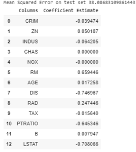
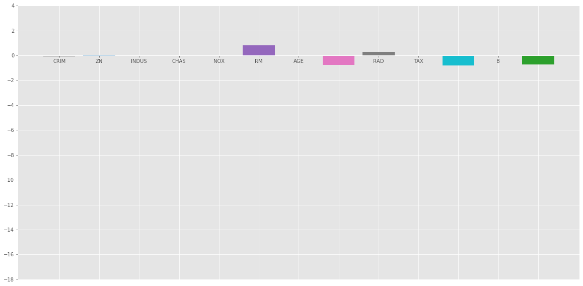
Output:

Elastic_Net

Bar plot of above coefficients:

Conclusion :
From the above analysis we can reach the following conclusion about different regularization methods:

Regularization is used to reduce the dependence on any particular independent variable by adding the penalty term to the Loss function. This term prevents the coefficients of the independent variables to take extreme values.
Ridge Regression adds L₂ regularization penalty term to loss function. This term reduces the coefficients but does not make them 0 and thus doesn’t eliminate any independent variable completely. It can be used to measure the impact of the different independent variables.
Lasso Regression adds L₁ regularization penalty term to loss function. This term reduces the coefficients as well as makes them 0 thus effectively eliminate the corresponding independent variable completely. It can be used for feature selection etc.
Elastic Net is a combination of both of the above regularization. It contains both the L₁ and L₂ as its penalty term. It performs better than Ridge and Lasso Regression for most of the test cases.

Suggest improvement

Feature Encoding Techniques - Machine Learning

ML | MultiLabel Ranking Metrics - Coverage Error

Share your thoughts in the comments

Implementation of Lasso, Ridge and Elastic Net

Python3

Python3

Python3

Python3

Python3

Python3

Python3

Python3

Python3

Python3

Please Login to comment...

Similar Reads

What kind of Experience do you want to share?