Introduction of Statistical Data Distributions

Distribution simply means collection or gathering of data, or scores, on variable. Generally, all these scores are arranged in specific order from smallest to largest. Then these scores can be presented graphically. Many data comply with rules of well-known and highly understood functions of mathematics.

A function can usually fit data with some modifications and changes in parameters of functions. As soon as distribution function is known and identified, it can be used as shorthand for describing and calculating related quantities. These quantities can be likelihood of observations, and plotting relationship between observations in domain.

Distributions are generally described in terms of their density or density functions. Density functions are simply described as functions that explain how proportion of data or likelihood of proportion of observations change over wide range of distribution. Density functions are of two types –

• Probability Density Function (PDF) –
  It calculates probability of observing given value.
• Cumulative Density Function (CDF) –
  It calculates probability of an observation equal or less than value.

Both PDFs and CDFs are type of continuous functions. For discrete distribution, equivalent of PDF is called Probability Mass Function (PMF).

Types of Statistical Data Distributions :

1. Gaussian Distribution –
   It is named after Carl Friedrich Gauss. Gaussian Distribution is focus of much of field of statistics. It is also known as Normal Distribution. With use of Gaussian Distribution, data from different study fields can be described. Generally, Gaussian Distribution is described using two parameters :
   • Mean :
     It is denoted with Greek lowercase letter “mu”. It is expected value of distribution.

   • Variance :
     It is denoted with Greek lowercase letter “sigma” raised to second power (this is because units of variables are squared.). It generally describes spread of observation from mean.

     It is very common and easy to use normalized calculation of variance called Standard Deviation. Standard Deviation is denoted with Greek lowercase letter “sigma”. It generally describes normalized spread of observations from mean.

   Example –
   The example given below creates Gaussian PDF with sample space from -5 to 5, mean of 0, and standard deviation of 1. Such type of gaussian with these values of mean and standard deviation is called Standard Gaussian.

   Python Code for Line Plot of Gaussian Probability Density Function :

   # plot the gaussian pdf
   from numpy import arrange
   from matplotlib import pyplot
   from scipy.stats import norm
   # define the distribution parameters 
   sample_space= arange (-5, 5, 0.001)
   mean= 0.0
   stdev= 1.0
   # calculate the pdf
   pdf= norm.pdf (sample_space, mean, stdev)
   # plot
   pyplot.plot (sample_space, pdf)
   pyplot.show ()
   

   When we run above example, it creates lined plot that shows sample space in x-axis and likelihood of each value of Y-axis. Line plot generally shows and represents familiar bell shape for gaussian distribution.

   

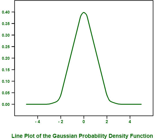
   In this plot, top of bell shows expected value or mean, which in this is zero, as we have already specified it while creating distribution.




2. T- Distribution –
   It is named after Willian Sealy Gosset. T- distribution generally arises when we attempt to find out mean of normal distribution with different sized samples. It is very helpful when describing uncertainty or error related to estimating or finding out population statistics for data drawn from Gaussian Distributions when size of sample must be considered. T-distribution can be described using single parameter.
   
   
   Number of Degrees of Freedom :
   It is denoted with Greek lowercase letter “nu (v)”. It simply denotes number of degrees of freedom. Number of degrees of freedom generally explains number of pieces of information that is used to describe population quantity.

   Example –
   The example given below creates t-distribution with sample space from -5 to 5 and (10, 000-1) degrees of freedom.

   Python Code for Line Plot of Student’s t-distribution Probability Density Function :

   # plot the t-distribution pdf
   from numpy import arange
   from matplotlib import pyplot
   from scipy.stats import t
   # define the distribution parameters 
   sample_space= arange (-5, 5, 0.001)
   dof= len(sample_space) - 1
   # calculate the pdf
   pdf= t.pdf (sample_space, dof)
   # plot
   pyplot.plot (sample_space, pdf)
   pyplot.show () 

   When we run above example, it creates and plots t-distribution PDF.

   

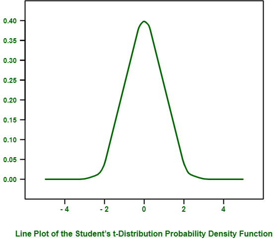
   You can see similar bell-shape to distribution much like normal. The main difference is fatter tails in distribution, highlighting increased likelihood of observations in tails as compared to that of Gaussian Distribution.