Iso-Probability Lines for Gaussian Processes Classification (GPC) in Scikit Learn

Gaussian Processes (GPs) are a powerful tool for probabilistic modeling and have been widely used in various fields such as machine learning, computer vision, and signal processing. Gaussian Processes Classification is a classification technique based on Gaussian Processes to model the probability of an input belonging to a certain class. In GPC, we assumed that the data is normally distributed.  In this article, we will explore the concept of Iso-Probability Lines and how they can be used to visualize the decision boundaries of GPC models in the Scikit Learn library.

Iso-Probability Lines

Iso-probability lines are contour lines on a plot that represents the same probability or likelihood of a given event or outcome. These lines are often used in classification problems to depict the boundary between different classes, with each line representing a different level of probability or confidence. They can also be used to represent the uncertainty or confidence of a prediction made by a model. The concept of iso-probability lines helps in visualizing the decision boundaries of a classifier and in understanding the behavior of a model.

Examples 1:

Step1: Import the necessary libraries

Step2: Generate data for classifications

With the help of make_classification from the sklearn.datasets module generates a random classification dataset. 

Step 3: Define kernel for GaussianProcessClassifier.

We will use the Radial Basis Function kernel

Output:

1**2 * RBF(length_scale=1)

Step 4: Define the Gaussian Process Classifier.

Define the Gaussian Process Classifier and fit the model.

Output:

GaussianProcessClassifier(kernel=1**2 * RBF(length_scale=1))

Step 5: Check the learned kernel by Gaussian Process Classifier.

Output:

10.7**2 * RBF(length_scale=3.74)

Step 6:  Creates a rectangular grid of points in 2D space to evaluate the Gaussian predicted probability

• np.linspace(-4, 4, 50) Create 50 points by dividing [-4,4] into 50 equal parts.
• np.meshgrid(k,k) will copy the same data horizontally and vertically and return two vectors respectively.
• Reshape the data and create (2500,2) array

Output:

Before Reshaping x1 : (50, 50)
Before Reshaping x2 : (50, 50)
After Reshaping  x1_ : (2500,)
After Reshaping  x2_ : (2500,)
Before Reshaping xx : (2, 2500)
After Reshaping  xx : (2500, 2)

array([[-4.        ,  0.89795918],
       [-3.83673469,  0.89795918],
       [-3.67346939,  0.89795918],
       [-3.51020408,  0.89795918],
       [-3.34693878,  0.89795918]])

Step 6: Predict the probability

Predict the Gaussian probability of the newly created dataset xx. it will result in the predictions in (2500,2) shape, where each row sum will be equal to 1.  we can either consider either the 1st or 2nd value by y_prob[:,0]  or y_prob[:,01]  and then reshape it into (50,50) shape to plot on the graph.

Output:

y_prob shape : (2500, 2)
check >> [ True  True  True ...  True  True  True]
y_prob shape : (50, 50)

Step 7: Plot the Graph with Iso-Probability Lines

The contour function in matplotlib is used to create a contour plot of a given function. It takes in 3 arguments: the x-coordinates, y-coordinates, and the function values at each point. In this code, the x-coordinates and y-coordinates are provided by the meshgrid created from the x and y ranges of the data points, and the function values are provided by the predict_proba method of the GPC model. 

The next step is to plot the probabilistic classification iso-values. This is done using the plt.contour() function from the matplotlib.pyplot library. The x1, x2, and y_prob arrays are passed as arguments to the function, along with the value of the iso-value (0.5). The colors and line styles arguments are also set to “k” and “dashed” respectively. The scatter() function is also used to plot the original dataset points, passing the X, y and cmap arguments.

Finally, the iso-probability lines are plotted using the plt.contour() function again, this time passing a list of values as the argument for the levels [0.1, 0.35, 0.65, 0.9]. The clabel() function is used to display the level values on the contour lines. The plot is shown using the plt.show() function.

Output:

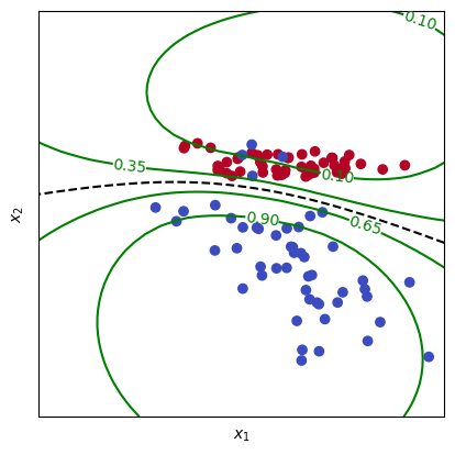
Iso-probability lines

Example 2:

The following steps may be followed in order to plot iso-probability lines for GPC in scikit-learn:

1. Import the necessary libraries and modules.
2. Load and preprocess the dataset.
3. Instantiate the GPC model using scikit-learn.
4. Fit the model to the data.
5. Plot the Iso-Probability Lines using matplotlib. 

Output:

Learned Kernel : 52.3**2 * RBF(length_scale=[2.29, 4.49])

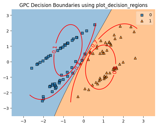
Iso-probability lines

This code uses the Gaussian Process Classification (GPC) algorithm from the scikit-learn library to classify a dataset of 100 samples, each with 2 informative features. The GPC algorithm is a probabilistic approach to classification, which makes use of Gaussian processes to model the underlying distribution of the data.

First, the code imports the necessary libraries, including scikit-learn’s GaussianProcessClassifier and RBF kernel, as well as numpy, matplotlib, and the plot_decision_regions function from mlxtend.

Next, the code generates a dataset of 100 samples using the make_classification function from scikit-learn’s datasets module. This function generates a random dataset of samples with binary labels.

The code then creates an instance of the GaussianProcessClassifier, and sets the kernel to a radial basis function (RBF) kernel with parameters 1.0, 1.0. The kernel is a crucial component of the GPC algorithm, as it defines the similarity between samples. The RBF kernel is a popular choice for GPC, as it allows for smooth decision boundaries.

Then, the code fits the model to the generated data set (X, y) using the gpc.fit(X, y) function

Then the code plots the decision regions using the plot_decision_regions function from the mlxtend library. This function generates a scatter plot of the input data, and shades each region with the predicted class label.

Next, the code creates a meshgrid of points to evaluate the model on using the numpy’s linspace function, this is done to have a fine grid of points to evaluate the model on.

The code then evaluates the model’s predict_proba method on each point of the meshgrid using gpc.predict_proba(xx). predict_proba returns the probability of each class for each sample.

ravel: This is a function from the NumPy module that returns a 1D array containing all the elements of the input array. It is used to flatten the 2D grid created by the meshgrid function so that it can be passed as input to the predict_proba method.

Then the code reshapes the y_prob by reshaping it to the shape of x1 and x2 , this is done to plot the probabilistic classification iso-values

Then the code plots the iso-probability lines using the contour function from matplotlib. The contour function generates a contour plot of the input data, with the levels parameter set to the desired iso-probability levels, in this case, 0.1, 0.2, 0.3, 0.4, 0.5, 0.6, 0.7, 0.8, 0.9.

Finally, the code displays the plot using plt.show() function

Example 3: 

Output:

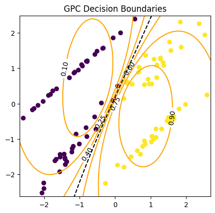
Iso-probability lines 

The code is a demonstration of how to use the Gaussian Process Classifier (GPC) from the scikit-learn library to create decision boundaries for a binary classification problem. The steps taken in the code are:

Import the necessary libraries: sklearn.gaussian_process, sklearn.gaussian_process.kernels, sklearn.datasets, matplotlib.pyplot, and numpy.

Generate a binary classification dataset using the make_classification() function from sklearn.datasets with 100 samples, 2 informative features, and a random state of 42. The variables X and y store the feature matrix and target vector, respectively.

Instantiate the GPC model using the Radial Basis Function (RBF) kernel and a random state of 42. The kernel is initialized with a scaling factor of 1 and a length-scale of 1 for both features.

Fit the GPC model to the data using the fit() method.

Create a meshgrid of points to evaluate the model by finding the minimum and maximum values of both features in the feature matrix X, and then creating a grid of 100×100 points between these values using the np.meshgrid() function.

Evaluate the model’s predict_proba() method on each point of the meshgrid by flattening the meshgrid points into a single array using np.c_[] and calling predict_proba() on it. The output of this function is an array of probability estimates for each point in the meshgrid, where the probability of the first class is in the first column and the probability of the second class is in the second column. In this case, the second column is selected and reshaped to match the shape of the meshgrid.

Create a contour plot of the decision boundaries using the plt.contour() function, where the x and y axis correspond to the points on the meshgrid, and the z-axis corresponds to the probability estimates. The contour levels are set to be at 0.1, 0.2, …, 0.9.

Plot the data points on top of the contour plot using the plt.scatter() function.

Set the aspect ratio of the plot to be equal and enable adjustable box.

Show the plot using the plt.show() function.

In conclusion, Gaussian Process Classification (GPC) is a powerful probabilistic classification method that can be used to model non-linear relationships between inputs and outputs. GPCs are particularly useful in situations where the underlying relationship between inputs and outputs is not well understood, and can be used in a wide range of applications, including image classification and object recognition. This article explores  how to use GPCs to create iso-probability lines, which can be used to visualize the decision boundary of the classifier. It is important to note that GPCs are computationally expensive and may not be suitable for large datasets. However, they can be a powerful tool in the right situations.