Laplacian of Gaussian Filter in MATLAB

The Laplacian filter is used to detect the edges in the images. But it has a disadvantage over the noisy images. It amplifies the noise in the image. Hence, first, we use a Gaussian filter on the noisy image to smoothen it and then subsequently use the Laplacian filter for edge detection.

Dealing with a noisy image without a Gaussian Filter:

Function used

• imread( ) is used for image reading.
• rgb2gray( ) is used to get gray image.
• conv2( ) is used for convolution.
• imtool( ) function is used to display the image.

Example:

Output:  

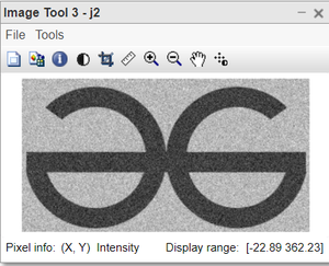
Figure: Input Noisy image

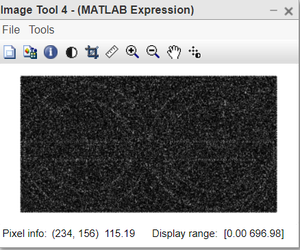
Figure: Edge detected image

Explanation of Code: 

• j=imread(“logo.png”);  This line Reads the image in MatLab
  Extension of the image can be anything i.e jfif, png, jpg, jpeg, etc.
• j1=rgb2gray(j); This line converts the image in grayscale, we avoid dealing with colored images.
  This function takes only one parameter and returns back the gray image.
• n=25*randn(size(j1)); This line generates the noise of size equal to gray image.
  Gaussian noise is additive in nature, so added directly using +.
• j2=n+double(j1); This line Generates noisy images by adding noise to the grayscale image.
• imtool(j,[]); This line display the original color image.
• imtool(j1,[]); This line display the gray image.
• imtool(j2,[]); This line display the noisy image.
• Lap=[0 -1 0; -1 4 -1; 0 -1 0]; This line of code define the Laplacian Filter.
• j3=conv2(j2, Lap, ‘same’); This line Convolve the noisy image with Laplacian filter.
  conv2( ) performs the convolution. It takes 3 parameters. ‘same’ ensures that result has the same size as of input image.
• imtool(abs(j3), []); This line display the resultant image.

Dealing with a noisy image using LOG:

Logarithmic transformation of an image is one of the gray-level image transformations. Log transformation of an image means replacing all pixel values, present in the image, with its logarithmic values. Log transformation is used for image enhancement as it expands dark pixels of the image as compared to higher pixel values.

Example:

 
Output: 

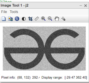
Figure: Input Noisy image

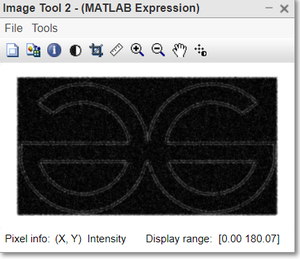
Figure: Edge detected image

Explanation of Code:

• j=imread(“logo.png”);  This line Reads the image in MatLab
  image is stored in variable j.
• j1=rgb2gray(j); This line converts the image in grayscale, we avoid dealing with colored images.
  j1 is the gray image and j is the color image.
• n=25*randn(size(j1)); This line generates the noise of size equal to gray image.
  random Gaussian noise is created.
• j2=n+double(j1); This line Generates noisy images by adding noise to the grayscale image.
  due to the addictive nature of gaussian noise, it has been directly added to the image.
• Gaussian=fspecial(‘gaussian’, 5, 1); This line creates the gaussian Filter.
  5 is the mean and 1 is the variance of the gaussian filter.
• Lap=[0 -1 0; -1 4 -1; 0 -1 0]; This line of code define the Laplacian Filter.
• j4=conv2(j2, Gaussian, ‘same’); This line Convolves the noisy image with Gaussian Filter first.
• j5=conv2(j4, Lap, ‘same’); This line Convolves the resultant image with Laplacian filter.
• imtool(j4,[]); This line displays the Gaussian of noisy_image.
• imtool(j5,[]); This line Displays the Laplacian of Gaussian resultant image.