Liveliness Analysis in Compiler Design

Liveliness Analysis consists of a specified technique that is implemented to optimize register space allocation, for a given piece of code and facilitate the procedure for dead-code elimination. As any machine has a limited number of registers to hold a variable or data which is being used or manipulated, there exists a need to balance out the efficient allocation of memory to reduce cost and also enable the machine to handle complex code and a considerable amount of variables at the same time. The procedure is carried out during the compilation of an input code by a compiler itself.

Live Variable: A variable is live at any instant of time, during the process of compilation of a program if its value is being used to process a computation as the evaluation of an arithmetic operation at that instant or it holds a value that will be used in the future without the variable being re-defined at any intermediate step.

Live Range: The live range of a variable is defined as the portion of code for which a variable was live. The live range of a variable might be continuous or distributed across different portions of the code. This implies that a variable might be live in an instant and dead in the next and might be live again for a certain portion. 

Liveliness Algorithm is used to evaluate the liveliness of each variable at each step. If one or more variables are live during the execution of a statement, the algorithm adds the evaluation to final result and repeats the same procedure for next statement. The output of the algorithm is further used to analyse the live range of variables and if any two variables are not live simultaneously at any instant of time, they share a common register. Hence, as a result, the available space is utilised effectively which is the motivation behind the algorithm.

The basic concept is derived from the fact that for a few temporary variables, the variables with disjoint live ranges can be put into a specific register, accordingly as and when they are needed. To ensure an appropriate allocation of a register to multiple variables, in accordance with the code, the concept of Liveliness Algorithm and Live Variable is introduced.

Terminologies Used:

Some key terminologies are as discussed below:

1. Control Flow Graph: A Control Flow Graph is described as a graphical form of representation for the flow control of a program through a directed graph, during the process of parsing. Each node of a Control Flow Graph (CFG) represents a single statement or a set of statements and each directed edge of the graph represents the control flow for the given code.

Note that, for a Control Flow Graph:

The outgoing edges point to a successor node.

succ[n] : It is the set of all successors of node 'n'.

The incoming edges arise from a predecessor node.

pred[n] : It is the set of all predecessors of node 'n'.

2. Data Flow Analysis: A procedure to extract key information about and learn the dynamic behavior of a given program by reviewing and analyzing the static code only.

3. Basic Block: The procedure to gather the liveliness information is a form of data flow analysis, operating over the Control Flow Graph where each statement, in general, is considered as a different Basic Block.

It is important to note that liveliness is a property of a variable which flows through and around the directed edges of the control flow graph.

4. Define a Variable: An assignment expression defines a variable, let’s say v, where a value is being assigned to v.

• def(v): It is defined as the set of all the nodes in the control flow graph where ‘v’ is defined.
• def[n]: It is defined as the set of variables defined by ‘n’, where ‘n’ is a node in the control flow graph and ‘v’ is a variable.

5. Use a Variable: Each occurrence of v in any number of expressions is said to be a use for the value of v being used for each statement which uses the value of ‘v’.

• use(v): It is defined as the set of all the nodes in the control flow graph that use ‘v’, and
• use[n]: It is the set of variables used in ‘n’, where ‘n’ is a node in the control flow graph and ‘v’ is a variable.

Note that use[n] and def[n] for a given node, are both independent of the control flow and hence are constants for each node, irrespective of the iterations.

6. Live: A variable ‘v’ is live on edge ‘e’ if there exists a directed path from the edge ‘e’ to use of ‘v’ that does not pass through any def(v).

7. Live-In: A variable ‘v’ is live-in at node ‘n’ if the variable is live on any of n’s in-edges.

8. Live-Out: A variable ‘v’ is live-out at a node ‘n’ if live on any of n’s out-edges.

To evaluate Live-In and Live-Out, we define

-> in[n]: As set of all the variables live-in at 'n' and
-> out[n]: As set of all the variables live-out at 'n',
where both in[n] and out[n] are initialised to NULL.

Note:

1. If a variable is used at a program statement that exists in a node, then the variable is live-in at that node. The definition is expressed as an expression below:

v ∈ use[n] ⇒ v live-in at n

2. In general, we assume that all the variables have been initialized beforehand. Also if a variable is live-in at a given node, then it is live-out at all of the predecessor nodes are directed to the node in a CFG.

v live-in at n ⇒ v live-out at all m ∈ pred[n]

3. A variable ‘v’, is alive at a given point of a program expressed as a node as ‘n’ if there exists a directed path from ‘n’ to use of ‘v’ and the path does not contain any definition of ‘v’.

v live-out at n, v ∉ def[n] ⇒ v live-in at n

Liveliness Algorithm:

The Liveliness Algorithm must execute the required functionality and an overview for the steps included in the algorithm design are as follows:

1. The first step is to identify which variables are defined and which ones are read (used) by instruction or a program statement by analyzing each node, step by step, in a CFG.  Also, initialize the value for IN and OUT to NULL. Note that Step-1 is executed only once.
2. Maintain global information record which aims at specifying how instructions transmit live values around the program and compute IN and OUT sets from def and use sets by using the expressions.
3. Now, iterate (2) until IN and OUT sets become constant for successive iterations. Remember that def and use sets are constants and hence path independent!

The Liveliness Algorithm is as follows:

N : Set of nodes of CFG;
for each n ∈ N do
    in[n] ← φ;
    out[n] ← φ;
end
repeat
      for each n ∈ Nodes do
          // First save the current value for IN and OUT for comparison later.
        in'[n] ← in[n];
        out'[n] ← out[n];        
        // For OUT, find out the union of previous variables 
            in the IN set for each succeeding node of n.
        out[n] ← ∪s∈succ[n]in[s] ; // Compute OUT for a node.
        in[n] ← use[n]∪(out[n]−def [n]); // Compute IN for a node.
    end
// Iterate, until IN and OUT set are constants for last two consecutive iterations.
until ∀n,in'[n] = in[n] ∧ out' [n] = out[n]; 

Liveliness Algorithm Analysis by an Example:

Problem: A variable x is said to be live at a statement Si in a program if the following three conditions hold simultaneously:

1. There exists a statement Sj that uses x
2. There is a path from Si to Sj in the flow graph corresponding to the program
3. The path has no intervening assignment to x including at Si and Sj

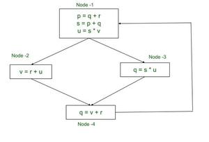
Control Flow Graph (Liveliness Analysis Example)

Solution: 

For the 1st Iteration, as we begin the procedure with Node-4 we have OUT and IN set to ∅. OUT and IN are empty sets as of now. Now OUT[n] is evaluated by using the expression ∪_s∈succ[n]in[s] and as Node-4 is succeeded by Node-1, we have :

Using , out[n] ← ∪s∈succ[n]in[s] , we have 
OUT2[4] ← IN2[1]  
OUT2[4] ← ∅

It is important to note that IN₂[1] has not been evaluated yet for the 1st iteration. Here, we only use the initial value for IN₂[1] , which is same as IN₁[1] and that is Empty Set. Later, when the value is evaluated by procedure, the result is updated to the table as well.

Similarly, we evaluate IN₂[4] as follows:

in[n] ← use[n]∪(out[n]−def [n])
IN2[4] ← use[4]∪(OUT2[4]-def[4])
We know, use[4]← {v,r} , OUT2[4] is ∅ & def[4] ← {q}
IN2[4] ← {v,r}∪( ∅ - {q} )
IN2[4] ← {v,r}

Let us evaluate IN and OUT for Node-1 which is succeeded by Node-2 and Node-3, as follows:

Using , out[n] ← ∪s∈succ[n]in[s] , we have
OUT2[1] ← IN2[2] ∪ IN2[3]  
OUT2[1] ← {s, u, r, v} ∪ {r, u}
OUT2[1] ← { s, u, r, v}

Now we evaluate IN₂[1] as follows:

in[n] ← use[n]∪(out[n]−def [n])
IN2[1] ← use[1]∪(OUT2[1]-def[1])
We know, use[1]← {q, r, v} , OUT2[1] is {s,u,r,v} & def[1] ← {p,s,u}
IN2[1] ← {q,r,v}∪( {s,u,r,v}- {p,s,u})
IN2[1] ← {q,r,v}∪( {r,v} )
IN2[1] ← {q,r,v}

Also, note that for the next iteration, OUT for Node-4 is evaluated as follows:

Using , out[n] ← ∪s∈succ[n]in[s] , we have
OUT3[4] ← IN3[1] 
Note that we use the already evaluated value of IN. 
As we begin with Node-4 we use IN3[1] = IN2[1].
IN2[1] is as calculated above.
OUT3[4] ← { q, r ,v}

The procedure is terminated after the 3^rd Iteration as the value for each resultant set for the last two iterations is exactly the same.

Time Complexity Analysis:

For input program of size N, ≤ N nodes in CFG and ≤ N variables we have :

1. N elements per in/out and hence, for the worst-case we have, O(N) time per set-union.
2. Note that the for loop performs a constant number of set operations per node and hence, O(N²) is the total time complexity for the loop.
3. The sizes of all IN and OUT set sum to 2N²  which is bounding the number of iterations of the repeat loop
4. We can evaluate the worst-case time complexity of the Liveliness Algorithm as O(N⁴).
5. It is important to note that appropriate ordering and use of an efficient data structure can cut the repeat loop down to 2-3 iterations.
6. We may conclude that the minimum possible worst-case time complexity of the Liveliness Algorithm is O(N) or O(N²).