Long short-term memory (LSTM) RNN in Tensorflow
Last Updated :
10 Jan, 2023
This article discusses the concept of “Recurrent Neural Networks(RNN)” and “Long Short Term Memory(LSTM)” and their implementation using Python programming language and the necessary library.
RECURRENT NEURAL NETWORK
- It is one of the oldest networks which was created in the year the 1980s but at the time there is no computation power of computers so it hasn’t come into the limelight in recent years it became very popular due to highly generated data and the high computation power of computers.
- The main use of RNN is it is very accurately used for sequence and time series data.
- It is one of the most powerful algorithms where it has internal memory to store previous data. This is one of the main key features in the structure of RNN.
- Internal memory helps to remember important things and this also allows one to predict what comes next RNN is a “Feedback” neural network where it has self-loops at the hidden layer.
- RNN has short-term memory which stores only a short span of information.
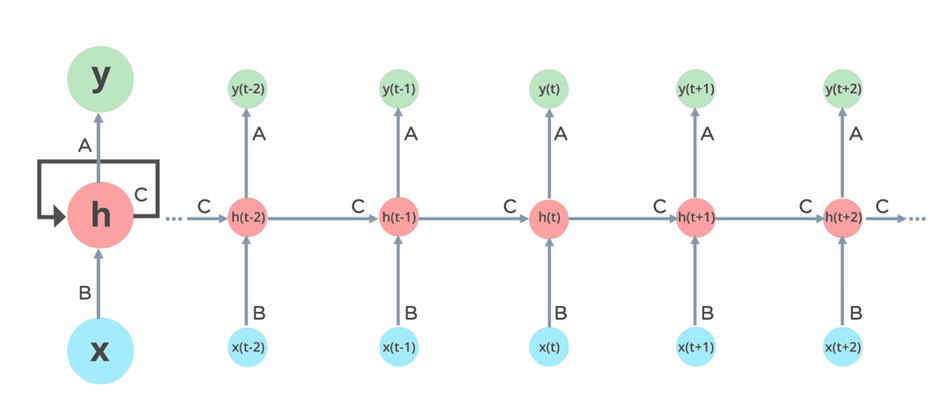
Architecture or RNN
The above architecture describes the RNN functionality we can observe input(x) is passing to the hidden layer(c) where the hidden layer has the self-loop to store the memory and the information passes to the output layer. Here the functionality of the hidden layer will be the next set of inputs so that the hidden layers act as short-term memory and carries the information to the next set of layers.
Drawbacks in RNN
- The computation will be slow
- The RNN networks only carry short-term information long term information can’t be taken into accommodation.
- It tends to vanish gradient problem(Value is too small and the model stops learning)
LONG SHORT-TERM MEMORY
To overcome the drawbacks encounters in RNN the scientist made an invention called “LONG SHORT TERM MEMORY”. LSTM is the child of RNN where it can store long-term information and overcome the drawback of vanishing gradient.
1. Forget Gate
It is responsible for keeping the information or forgetting it so the sigmoid activation function is applied to it the output will be ranging from 0-1 if it is 0(forget the information) or 1(keep the information).
2. Input Gate
It is responsible for expressing the importance of new information carried by the input here we will be applying two activation functions sigmoid and tanh. Sigmoid functionality is to keep or discard the information whereas tanh function is to subtract information from the cell state or to add new information to the cell state.
3. Output gate
Based on the information we have gained we give our sentence as the fill-in-the-blank to the output gate based on the information it perceived will output the result
Importing Libraries and Dataset
Python libraries make it very easy for us to handle the data and perform typical and complex tasks with a single line of code.
- Pandas – This library helps to load the data frame in a 2D array format and has multiple functions to perform analysis tasks in one go.
- Numpy – Numpy arrays are very fast and can perform large computations in a very short time.
- Matplotlib – This library is used to draw visualizations.
- NLTK – Natural Language Tool Kit is a very handy tool that is used to transform raw text into processed one so, that it can be fed into a Machine Learning model.
- TensorFlow – This is an open-source library that is used for Machine Learning and Artificial intelligence and provides a range of functions to achieve complex functionalities with single lines of code.
Python3
import pandas as pd
import numpy as np
import matplotlib.pyplot as plt
import seaborn as sns
from tensorflow import keras
from keras.models import Sequential
from keras.layers import Dense
from keras.layers import LSTM
|
Step 2: Now load the data using the pandas dataframe. We will use milk production data in this article which you can download from here.
Python
df = pd.read_csv('monthly_milk_production.csv',
index_col='Date',
parse_dates=True)
df.index.freq = 'MS'
|
Now let’s check whether the dataset has been loaded properly or not by printing the first five rows of the dataset.
Output:
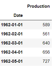
First five rows of the dataset
Step 4: Now proceed to perform EDA analysis on the dataset.
Output:
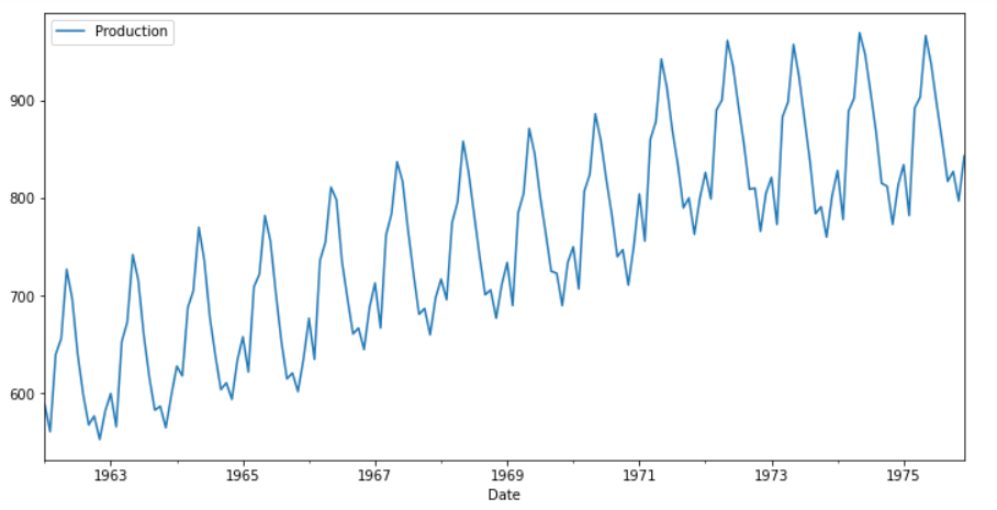
The trend in milk production over time
Step 5: Seasonal analysis of the time series data.
Python3
from statsmodels.tsa.seasonal import seasonal_decompose
results = seasonal_decompose(df['Production'])
results.plot()
|
Output:
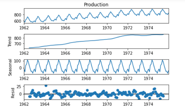
Seasonal, Trend, and Residuals graphs in the provided data
Step 6:- Splitting the data into training and testing.
Python
train = df.iloc[:156]
test = df.iloc[156:]
|
Step 7: Scaling our data to perform computations in a fast and accurate manner.
Python3
from sklearn.preprocessing import MinMaxScaler
scaler = MinMaxScaler()
scaler.fit(train)
scaled_train = scaler.transform(train)
scaled_test = scaler.transform(test)
|
Step 8: Processing to a time series generation.
Python3
from keras.preprocessing.sequence import TimeseriesGenerator
n_input = 3
n_features = 1
generator = TimeseriesGenerator(scaled_train,
scaled_train,
length=n_input,
batch_size=1)
X, y = generator[0]
print(f'Given the Array: \n{X.flatten()}')
print(f'Predict this y: \n {y}')
n_input = 12
generator = TimeseriesGenerator(scaled_train,
scaled_train,
length=n_input,
batch_size=1)
|
Step 9: Now let’s define the architecture of the model using TensorFlow API.
Python3
model = Sequential()
model.add(LSTM(100, activation='relu',
input_shape=(n_input, n_features)))
model.add(Dense(1))
model.compile(optimizer='adam', loss='mse')
model.summary()
model.fit(generator, epochs=5)
|
Output:
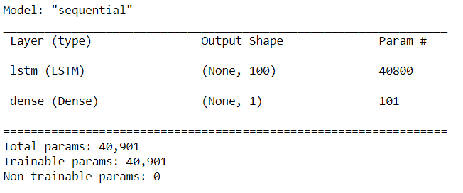
The architecture of the LSTM model
Step 10: Output the accuracy
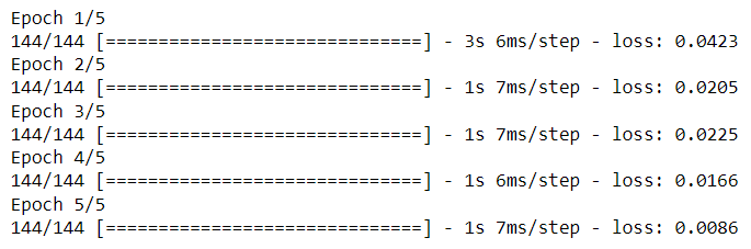
Training Progress of the LSTM model
Like Article
Suggest improvement
Share your thoughts in the comments
Please Login to comment...