Long Short Term Memory Networks Explanation
Last Updated :
02 Jan, 2023
Prerequisites: Recurrent Neural Networks
To solve the problem of Vanishing and Exploding Gradients in a Deep Recurrent Neural Network, many variations were developed. One of the most famous of them is the Long Short Term Memory Network(LSTM). In concept, an LSTM recurrent unit tries to “remember” all the past knowledge that the network is seen so far and to “forget” irrelevant data. This is done by introducing different activation function layers called “gates” for different purposes. Each LSTM recurrent unit also maintains a vector called the Internal Cell State which conceptually describes the information that was chosen to be retained by the previous LSTM recurrent unit.
LSTM networks are the most commonly used variation of Recurrent Neural Networks (RNNs). The critical component of the LSTM is the memory cell and the gates (including the forget gate but also the input gate), inner contents of the memory cell are modulated by the input gates and forget gates. Assuming that both of the segue he are closed, the contents of the memory cell will remain unmodified between one time-step and the next gradients gating structure allows information to be retained across many time-steps, and consequently also allows group that to flow across many time-steps. This allows the LSTM model to overcome the vanishing gradient properly occurs with most Recurrent Neural Network models.
A Long Short Term Memory Network consists of four different gates for different purposes as described below:-
- Forget Gate(f): At forget gate the input is combined with the previous output to generate a fraction between 0 and 1, that determines how much of the previous state need to be preserved (or in other words, how much of the state should be forgotten). This output is then multiplied with the previous state. Note: An activation output of 1.0 means “remember everything” and activation output of 0.0 means “forget everything.” From a different perspective, a better name for the forget gate might be the “remember gate”
- Input Gate(i): Input gate operates on the same signals as the forget gate, but here the objective is to decide which new information is going to enter the state of LSTM. The output of the input gate (again a fraction between 0 and 1) is multiplied with the output of tan h block that produces the new values that must be added to previous state. This gated vector is then added to previous state to generate current state
- Input Modulation Gate(g): It is often considered as a sub-part of the input gate and much literature on LSTM’s does not even mention it and assume it is inside the Input gate. It is used to modulate the information that the Input gate will write onto the Internal State Cell by adding non-linearity to the information and making the information Zero-mean. This is done to reduce the learning time as Zero-mean input has faster convergence. Although this gate’s actions are less important than the others and are often treated as a finesse-providing concept, it is good practice to include this gate in the structure of the LSTM unit.
- Output Gate(o): At output gate, the input and previous state are gated as before to generate another scaling fraction that is combined with the output of tanh block that brings the current state. This output is then given out. The output and state are fed back into the LSTM block.
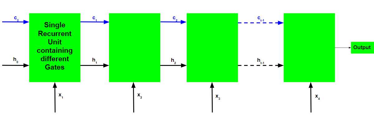
The basic workflow of a Long Short Term Memory Network is similar to the workflow of a Recurrent Neural Network with the only difference being that the Internal Cell State is also passed forward along with the Hidden State.
Working of an LSTM recurrent unit:
- Take input the current input, the previous hidden state, and the previous internal cell state.
- Calculate the values of the four different gates by following the below steps:-
- For each gate, calculate the parameterized vectors for the current input and the previous hidden state by element-wise multiplication with the concerned vector with the respective weights for each gate.
- Apply the respective activation function for each gate element-wise on the parameterized vectors. Below given is the list of the gates with the activation function to be applied for the gate.
- Calculate the current internal cell state by first calculating the element-wise multiplication vector of the input gate and the input modulation gate, then calculate the element-wise multiplication vector of the forget gate and the previous internal cell state and then add the two vectors.

- Calculate the current hidden state by first taking the element-wise hyperbolic tangent of the current internal cell state vector and then performing element-wise multiplication with the output gate.
The above-stated working is illustrated as below:-
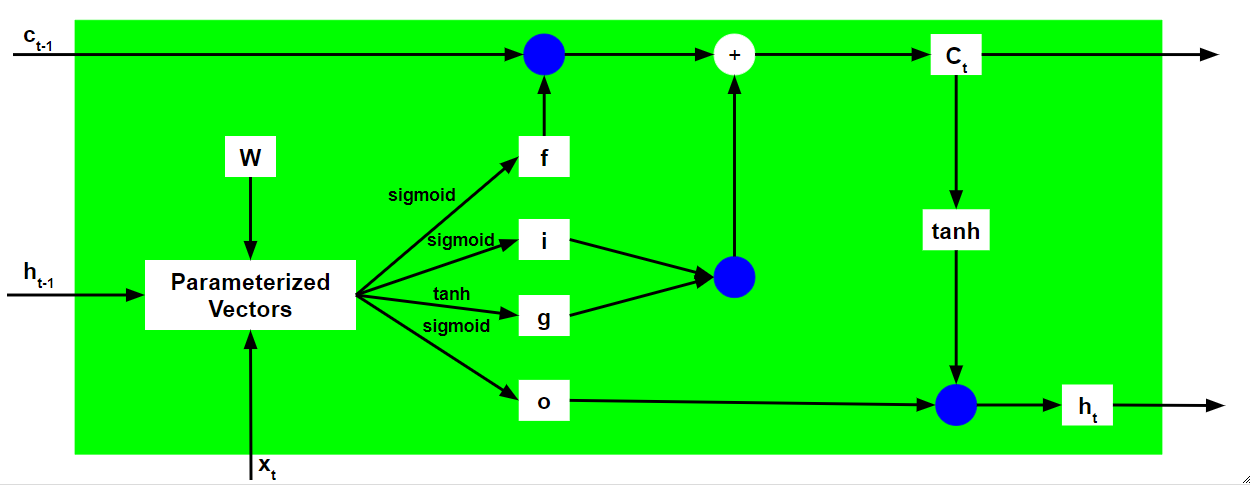
Note that the blue circles denote element-wise multiplication. The weight matrix W contains different weights for the current input vector and the previous hidden state for each gate.
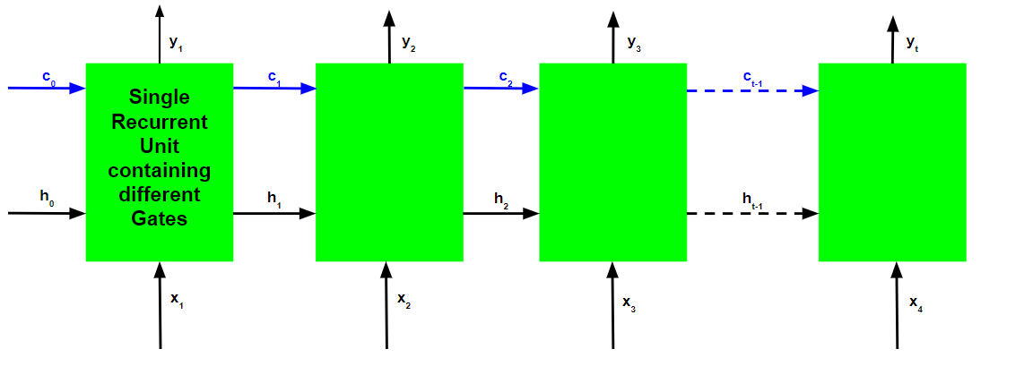
Just like Recurrent Neural Networks, an LSTM network also generates an output at each time step and this output is used to train the network using gradient descent.
The only main difference between the Back-Propagation algorithms of Recurrent Neural Networks and Long Short Term Memory Networks is related to the mathematics of the algorithm.
Let  be the predicted output at each time step and
  be the actual output at each time step. Then the error at each time step is given by:-

The total error is thus given by the summation of errors at all time steps.


Similarly, the value  can be calculated as the summation of the gradients at each time step.

Using the chain rule and using the fact that is a function of  and which indeed is a function of
  , the following expression arises:-

Thus the total error gradient is given by the following:-

Note that the gradient equation involves a chain of  for an LSTM Back-Propagation while the gradient equation involves a chain of
  for a basic Recurrent Neural Network.
How does LSTM solve the problem of vanishing and exploding gradients?
Recall the expression for .

The value of the gradients is controlled by the chain of derivatives starting from  . Expanding this value using the expression for :-

For a basic RNN, the term  after a certain time starts to take values either greater than 1 or less than 1 but always in the same range. This is the root cause of the vanishing and exploding gradients problem. In an LSTM, the term does not have a fixed pattern and can take any positive value at any time step. Thus, it is not guaranteed that for an infinite number of time steps, the term will converge to 0 or diverge completely. If the gradient starts converging towards zero, then the weights of the gates can be adjusted accordingly to bring it closer to 1. Since during the training phase, the network adjusts these weights only, it thus learns when to let the gradient converge to zero and when to preserve it.
Like Article
Suggest improvement
Share your thoughts in the comments
Please Login to comment...