The challenge is to recognize fraudulent credit card transactions so that the customers of credit card companies are not charged for items that they did not purchase.
Before going to the code it is requested to work on a jupyter notebook. If not installed on your machine you can use Google colab.
You can download the dataset from this link
If the link is not working please go to this link and login to kaggle to download the dataset.
Code : Importing all the necessary Libraries
import numpy as np
import pandas as pd
import matplotlib.pyplot as plt
import seaborn as sns
from matplotlib import gridspec
|
Code : Loading the Data
data = pd.read_csv("credit.csv")
|
Code : Understanding the Data
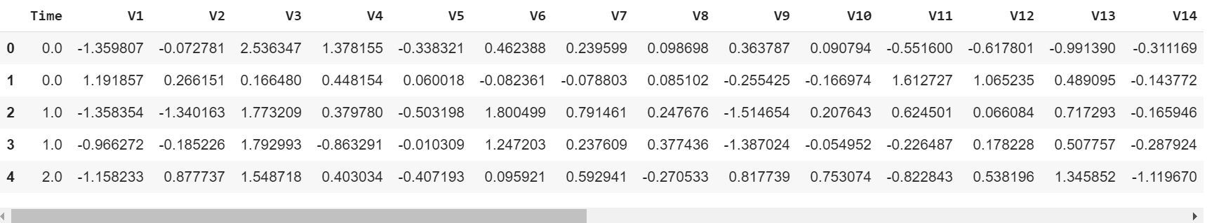
Code : Describing the Data
print(data.shape)
print(data.describe())
|
Output :
(284807, 31)
                Time            V1  ...         Amount          Class
count  284807.000000  2.848070e+05  ...  284807.000000  284807.000000
mean    94813.859575  3.919560e-15  ...      88.349619       0.001727
std     47488.145955  1.958696e+00  ...     250.120109       0.041527
min         0.000000 -5.640751e+01  ...       0.000000       0.000000
25%     54201.500000 -9.203734e-01  ...       5.600000       0.000000
50%     84692.000000  1.810880e-02  ...      22.000000       0.000000
75%    139320.500000  1.315642e+00  ...      77.165000       0.000000
max    172792.000000  2.454930e+00  ...   25691.160000       1.000000

[8 rows x 31 columns]
Code : Imbalance in the data
Time to explain the data we are dealing with.
fraud = data[data['Class'] == 1]
valid = data[data['Class'] == 0]
outlierFraction = len(fraud)/float(len(valid))
print(outlierFraction)
print('Fraud Cases: {}'.format(len(data[data['Class'] == 1])))
print('Valid Transactions: {}'.format(len(data[data['Class'] == 0])))
|
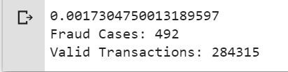
Only 0.17% fraudulent transaction out all the transactions. The data is highly Unbalanced. Lets first apply our models without balancing it and if we don’t get a good accuracy then we can find a way to balance this dataset. But first, let’s implement the model without it and will balance the data only if needed.
Code : Print the amount details for Fraudulent Transaction
print(“Amount details of the fraudulent transaction”)
fraud.Amount.describe()
|
Output :
Amount details of the fraudulent transaction
count     492.000000
mean      122.211321
std       256.683288
min         0.000000
25%         1.000000
50%         9.250000
75%       105.890000
max      2125.870000
Name: Amount, dtype: float64
Code : Print the amount details for Normal Transaction
print(“details of valid transaction”)
valid.Amount.describe()
|
Output :
Amount details of valid transaction
count    284315.000000
mean         88.291022
std         250.105092
min           0.000000
25%           5.650000
50%          22.000000
75%          77.050000
max       25691.160000
Name: Amount, dtype: float64
As we can clearly notice from this, the average Money transaction for the fraudulent ones is more. This makes this problem crucial to deal with.
Code : Plotting the Correlation Matrix
The correlation matrix graphically gives us an idea of how features correlate with each other and can help us predict what are the features that are most relevant for the prediction.
corrmat = data.corr()
fig = plt.figure(figsize = (12, 9))
sns.heatmap(corrmat, vmax = .8, square = True)
plt.show()
|
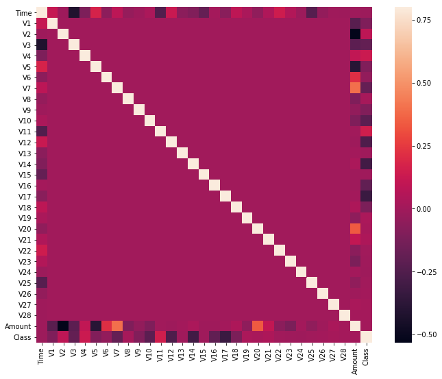
In the HeatMap we can clearly see that most of the features do not correlate to other features but there are some features that either has a positive or a negative correlation with each other. For example, V2 and V5 are highly negatively correlated with the feature called Amount. We also see some correlation with V20 and Amount. This gives us a deeper understanding of the Data available to us.
Code : Separating the X and the Y values
Dividing the data into inputs parameters and outputs value format
X = data.drop(['Class'], axis = 1)
Y = data["Class"]
print(X.shape)
print(Y.shape)
xData = X.values
yData = Y.values
|
Output :
(284807, 30)
(284807, )
Training and Testing Data Bifurcation
We will be dividing the dataset into two main groups. One for training the model and the other for Testing our trained model’s performance.
from sklearn.model_selection import train_test_split
xTrain, xTest, yTrain, yTest = train_test_split(
xData, yData, test_size = 0.2, random_state = 42)
|
Code : Building a Random Forest Model using scikit learn
from sklearn.ensemble import RandomForestClassifier
rfc = RandomForestClassifier()
rfc.fit(xTrain, yTrain)
yPred = rfc.predict(xTest)
|
Code : Building all kinds of evaluating parameters
from sklearn.metrics import classification_report, accuracy_score
from sklearn.metrics import precision_score, recall_score
from sklearn.metrics import f1_score, matthews_corrcoef
from sklearn.metrics import confusion_matrix
n_outliers = len(fraud)
n_errors = (yPred != yTest).sum()
print("The model used is Random Forest classifier")
acc = accuracy_score(yTest, yPred)
print("The accuracy is {}".format(acc))
prec = precision_score(yTest, yPred)
print("The precision is {}".format(prec))
rec = recall_score(yTest, yPred)
print("The recall is {}".format(rec))
f1 = f1_score(yTest, yPred)
print("The F1-Score is {}".format(f1))
MCC = matthews_corrcoef(yTest, yPred)
print("The Matthews correlation coefficient is{}".format(MCC))
|
Output :
The model used is Random Forest classifier
The accuracy is  0.9995611109160493
The precision is 0.9866666666666667
The recall is 0.7551020408163265
The F1-Score is 0.8554913294797689
The Matthews correlation coefficient is0.8629589216367891
Code : Visualizing the Confusion Matrix
LABELS = ['Normal', 'Fraud']
conf_matrix = confusion_matrix(yTest, yPred)
plt.figure(figsize =(12, 12))
sns.heatmap(conf_matrix, xticklabels = LABELS,
yticklabels = LABELS, annot = True, fmt ="d");
plt.title("Confusion matrix")
plt.ylabel('True class')
plt.xlabel('Predicted class')
plt.show()
|
Output :
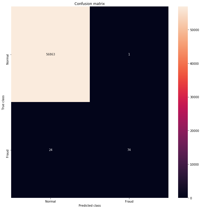
Comparison with other algorithms without dealing with the imbalancing of the data.
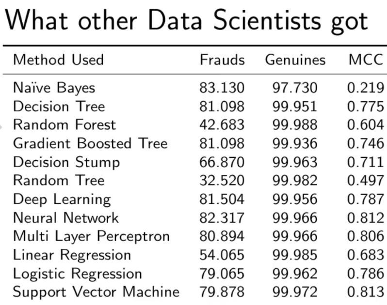
As you can see with our Random Forest Model we are getting a better result even for the recall which is the most tricky part.
Like Article
Suggest improvement
Share your thoughts in the comments
Please Login to comment...