OpenCV – The Gunnar-Farneback optical flow
Last Updated :
29 Nov, 2021
In this article, we will know about Dense Optical Flow by Gunnar FarneBack technique, it was published in a research paper named ‘Two-Frame Motion Estimation Based on Polynomial Expansion’ by Gunnar Farneback in 2003.
Prerequisites: OpenCV
Optical Flow:
Optical flow is known as the pattern of apparent motion of objects, i.e, it is the motion of objects between every two consecutive frames of the sequence, which is caused by the movement of the object being captured or the camera capturing it. Consider an object with intensity I (x, y, t), after time dt, it moves to by dx and dy, now, the new intensity would be, I (x+dx, y+dy, t+dt).
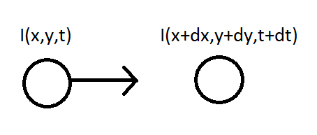
We, assume that the pixel intensities are constant between the two frames, i.e.,
I (x, y, t) = I (x+dx, y+dy, t+dt)
Taylor approximation is done on the RHS side, resulting in,
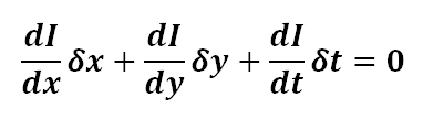
On dividing by δt, we obtain the Optical Flow Equation, i.e.,
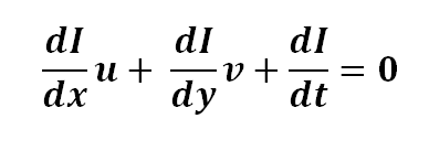
where, u = dx/dt and v = dy/dt.
Also, dI/dx is the image gradient along the horizontal axis, dI/dy is the image gradient along the vertical axis and dI/dt is along the time.
Since, we have just one equation to find two unknowns, we use different methods to solve,
Gunnar Farneback Optical Flow
In dense optical flow, we look at all of the points(unlike Lucas Kanade which works only on corner points detected by Shi-Tomasi Algorithm) and detect the pixel intensity changes between the two frames, resulting in an image with highlighted pixels, after converting to hsv format for clear visibility.
It computes the magnitude and direction of optical flow from an array of the flow vectors, i.e., (dx/dt, dy/dt). Later it visualizes the angle (direction) of flow by hue and the distance (magnitude) of flow by value of HSV color representation.For visibility to be optimal, strength of HSV is set to 255. OpenCV provides a function cv2.calcOpticalFlowFarneback to look into dense optical flow.
Syntax:
cv2.calcOpticalFlowFarneback(prev, next, pyr_scale, levels, winsize, iterations, poly_n, poly_sigma, flags[, flow])
Parameters:
- prev : First input image in 8-bit single channel format.
- next : Second input image of same type and same size as prev.
- pyr_scale : parameter specifying the image scale to build pyramids for each image (scale < 1). A classic pyramid is of generally 0.5 scale, every new layer added, it is halved to the previous one.
- levels : levels=1 says, there are no extra layers (only the initial image) . It is the number of pyramid layers including the first image.
- winsize : It is the average window size, larger the size, the more robust the algorithm is to noise, and provide fast motion detection, though gives blurred motion fields.
- iterations : Number of iterations to be performed at each pyramid level.
- poly_n : It is typically 5 or 7, it is the size of the pixel neighbourhood which is used to find polynomial expansion between the pixels.
- poly_sigma : standard deviation of the gaussian that is for derivatives to be smooth as the basis of the polynomial expansion. It can be 1.1 for poly= 5 and 1.5 for poly= 7.
- flow : computed flow image that has similar size as prev and type to be CV_32FC2.
- flags : It can be a combination of-
OPTFLOW_USE_INITIAL_FLOW uses input flow as initial approximation.
OPTFLOW_FARNEBACK_GAUSSIAN uses gaussian winsize*winsize filter.
Code:
Python3
import cv2
import numpy as np
capture = cv2.VideoCapture("video_file.avi")
_, frame1 = capture.read()
prvs = cv2.cvtColor(frame1, cv2.COLOR_BGR2GRAY)
hsv_mask = np.zeros_like(frame1)
hsv_mask[..., 1] = 255
while(1):
_, frame2 = capture.read()
next = cv2.cvtColor(frame2, cv2.COLOR_BGR2GRAY)
flow = cv2.calcOpticalFlowFarneback(prvs, next, None, 0.5, 3, 15, 3, 5, 1.2, 0)
mag, ang = cv2.cartToPolar(flow[..., 0], flow[..., 1])
hsv_mask[..., 0] = ang * 180 / np.pi / 2
hsv_mask[..., 2] = cv2.normalize(mag, None, 0, 255, cv2.NORM_MINMAX)
rgb_representation = cv2.cvtColor(hsv_mask, cv2.COLOR_HSV2BGR)
cv2.imshow('frame2', rgb_representation)
kk = cv2.waitKey(20) & 0xff
if kk == ord('e'):
break
elif kk == ord('s'):
cv2.imwrite('Optical_image.png', frame2)
cv2.imwrite('HSV_converted_image.png', rgb_representation)
prvs = next
capture.release()
cv2.destroyAllWindows()
|
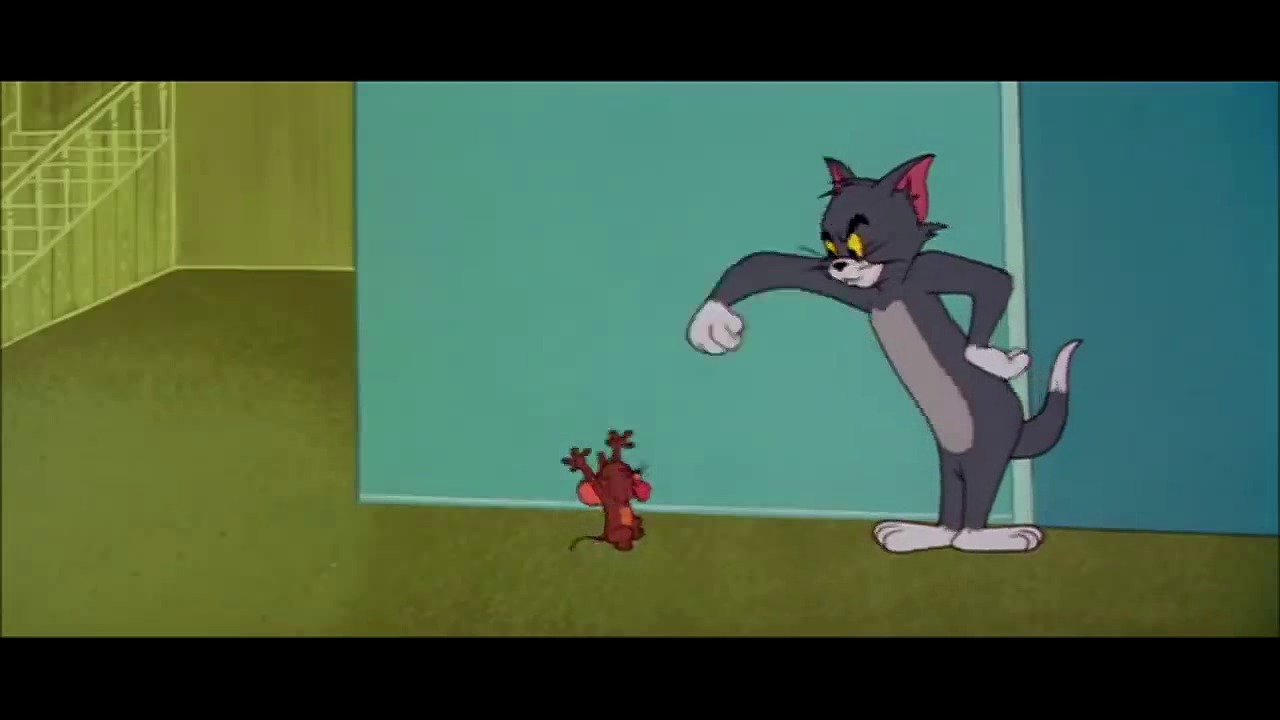
Input
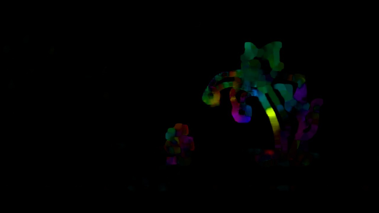
Output:
- https://docs.opencv.org/2.4/modules/video/doc/motion_analysis_and_object_tracking.html
Like Article
Suggest improvement
Share your thoughts in the comments
Please Login to comment...