Polynomial Regression in R Programming
Last Updated :
21 Jul, 2021
Polynomial Regression is a form of linear regression in which the relationship between the independent variable x and dependent variable y is modeled as an nth degree polynomial. Polynomial regression fits a nonlinear relationship between the value of x and the corresponding conditional mean of y, denoted E(y|x). Basically it adds the quadratic or polynomial terms to the regression. Generally, this kind of regression is used for one resultant variable and one predictor.
Need of Polynomial Regression
- Unlike linear data set, if one tries to apply linear model on non-linear data set without any modification, then there will be a very unsatisfactory and drastic result .
- This may lead to increase in loss function, decrease in accuracy and high error rate.
- Unlike linear model, polynomial model covers more data points.
Applications of Polynomial Regression
Generally, polynomial regression is used in the following scenarios :
- Rate of growth of tissues.
- Progression of the epidemics related to disease.
- Distribution phenomenon of the isotopes of carbon in lake sediments.
Explanation of Polynomial Regression in R Programming
Polynomial Regression is also known as Polynomial Linear Regression since it depends on the linearly arranged coefficients rather than the variables. In R, if one wants to implement polynomial regression then he must install the following packages:
- tidyverse package for better visualization and manipulation.
- caret package for a smoother and easier machine learning workflow.
After proper installation of the packages, one needs to set the data properly. For that, first one needs to split the data into two sets(train set and test set). Then one can visualize the data into various plots. In R, in order to fit a polynomial regression, first one needs to generate pseudo random numbers using the set.seed(n) function.
The polynomial regression adds polynomial or quadratic terms to the regression equation as follow:
medv = b0 + b1 * lstat + b2 * lstat 2
where
mdev: is the median house value
lstat: is the predictor variable
In R, to create a predictor x2 one should use the function I(), as follow: I(x2). This raise x to the power 2. The polynomial regression can be computed in R as follow:
lm(medv ~ lstat + I(lstat^2), data = train.data)
For this following example let’s take the Boston data set of MASS package.
Example:
r
library(tidyverse)
library(caret)
theme_set(theme_classic())
data("Boston", package = "MASS")
set.seed(123)
training.samples <- Boston$medv %>%
createDataPartition(p = 0.8, list = FALSE)
train.data <- Boston[training.samples, ]
test.data <- Boston[-training.samples, ]
model <- lm(medv ~ poly(lstat, 5, raw = TRUE),
data = train.data)
predictions <- model %>% predict(test.data)
modelPerfomance = data.frame(
RMSE = RMSE(predictions, test.data$medv),
R2 = R2(predictions, test.data$medv)
)
print(lm(medv ~ lstat + I(lstat^2), data = train.data))
print(modelPerfomance)
|
Output:
Call:
lm(formula = medv ~ lstat + I(lstat^2), data = train.data)

Coefficients:
(Intercept)        lstat     I(lstat^2)
    42.5736       -2.2673       0.0412

      RMSE        R2
1   5.270374 0.6829474
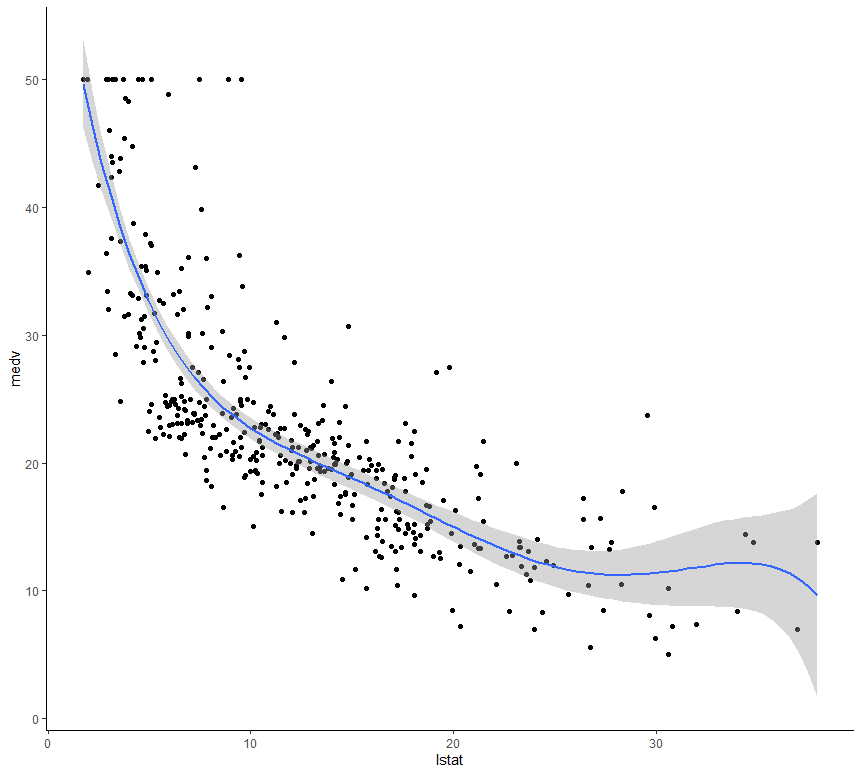
Graph plotting of Polynomial Regression
In R, if one wants to plot a graph for the output generated on implementing Polynomial Regression he can use the ggplot() function.
Example:
r
library(tidyverse)
library(caret)
theme_set(theme_classic())
data("Boston", package = "MASS")
set.seed(123)
training.samples <- Boston$medv %>%
createDataPartition(p = 0.8, list = FALSE)
train.data <- Boston[training.samples, ]
test.data <- Boston[-training.samples, ]
model <- lm(medv ~ poly(lstat, 5, raw = TRUE), data = train.data)
predictions <- model %>% predict(test.data)
data.frame(RMSE = RMSE(predictions, test.data$medv),
R2 = R2(predictions, test.data$medv))
ggplot(train.data, aes(lstat, medv) ) + geom_point() +
stat_smooth(method = lm, formula = y ~ poly(x, 5, raw = TRUE))
|
Output:
Like Article
Suggest improvement
Share your thoughts in the comments
Please Login to comment...