Recurrent Neural Networks Explanation

Today, different Machine Learning techniques are used to handle different types of data. One of the most difficult types of data to handle and the forecast is sequential data. Sequential data is different from other types of data in the sense that while all the features of a typical dataset can be assumed to be order-independent, this cannot be assumed for a sequential dataset. To handle such type of data, the concept of Recurrent Neural Networks was conceived. It is different from other Artificial Neural Networks in its structure. While other networks “travel” in a linear direction during the feed-forward process or the back-propagation process, the Recurrent Network follows a recurrence relation instead of a feed-forward pass and uses Back-Propagation through time to learn. 

The Recurrent Neural Network consists of multiple fixed activation function units, one for each time step. Each unit has an internal state which is called the hidden state of the unit. This hidden state signifies the past knowledge that the network currently holds at a given time step. This hidden state is updated at every time step to signify the change in the knowledge of the network about the past. The hidden state is updated using the following recurrence relation:- 



 

[Tex]- The new hidden state[/Tex][Tex]- The old hidden state[/Tex][Tex]- The current input[/Tex][Tex]- The fixed function with trainable weights[/Tex]

Note: Typically, to understand the concepts of a Recurrent Neural Network, it is often illustrated in its unrolled form and this norm will be followed in this post. 

At each time step, the new hidden state is calculated using the recurrence relation as given above. This new generated hidden state is used to generate indeed a new hidden state and so on. 

The basic work-flow of a Recurrent Neural Network is as follows:- 

 

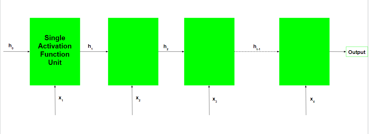
Note that is the initial hidden state of the network. Typically, it is a vector of zeros, but it can have other values also. One method is to encode the presumptions about the data into the initial hidden state of the network. For example, for a problem to determine the tone of a speech given by a renowned person, the person’s past speeches’ tones may be encoded into the initial hidden state. Another technique is to make the initial hidden state a trainable parameter. Although these techniques add little nuances to the network, initializing the hidden state vector to zeros is typically an effective choice. 

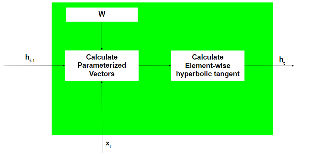
Working of each Recurrent Unit: 
 

1. Take input the previously hidden state vector and the current input vector. 
   
   Note that since the hidden state and current input are treated as vectors, each element in the vector is placed in a different dimension which is orthogonal to the other dimensions. Thus each element when multiplied by another element only gives a non-zero value when the elements involved are non-zero and the elements are in the same dimension.
2. Element-wise multiplies the hidden state vector by the hidden state weights and similarly performs the element-wise multiplication of the current input vector and the current input weights. This generates the parameterized hidden state vector and the current input vector. 
   
   Note that weights for different vectors are stored in the trainable weight matrix.
3. Perform the vector addition of the two parameterized vectors and then calculate the element-wise hyperbolic tangent to generate the new hidden state vector.

 

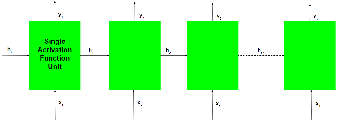
During the training of the recurrent network, the network also generates an output at each time step. This output is used to train the network using gradient descent. 

 

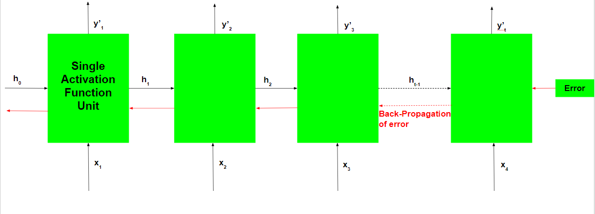
The Back-Propagation involved is similar to the one used in a typical Artificial Neural Network with some minor changes. These changes are noted as:- 

Let the predicted output of the network at any time step be and the actual output be . Then the error at each time step is given by:- 




The total error is given by the summation of the errors at all the time steps. 






Similarly, the value can be calculated as the summation of gradients at each time step. 




Using the chain rule of calculus and using the fact that the output at a time step t is a function of the current hidden state of the recurrent unit, the following expression arises:- 




Note that the weight matrix W used in the above expression is different for the input vector and hidden state vector and is only used in this manner for notational convenience. 

Thus the following expression arises:- 




Thus, Back-Propagation Through Time only differs from a typical Back-Propagation in the fact the errors at each time step are summed up to calculate the total error. 

 

Although the basic Recurrent Neural Network is fairly effective, it can suffer from a significant problem. For deep networks, The Back-Propagation process can lead to the following issues:- 
 

• Vanishing Gradients: This occurs when the gradients become very small and tend towards zero.
• Exploding Gradients: This occurs when the gradients become too large due to back-propagation.

The problem of Exploding Gradients may be solved by using a hack – By putting a threshold on the gradients being passed back in time. But this solution is not seen as a solution to the problem and may also reduce the efficiency of the network. To deal with such problems, two main variants of Recurrent Neural Networks were developed – Long Short Term Memory Networks and Gated Recurrent Unit Networks.

Recurrent Neural Networks (RNNs) are a type of artificial neural network that is designed to process sequential data. Unlike traditional feedforward neural networks, RNNs can take into account the previous state of the sequence while processing the current state, allowing them to model temporal dependencies in data.

The key feature of RNNs is the presence of recurrent connections between the hidden units, which allow information to be passed from one time step to the next. This means that the hidden state at each time step is not only a function of the input at that time step, but also a function of the previous hidden state.

In an RNN, the input at each time step is typically a vector representing the current state of the sequence, and the output at each time step is a vector representing the predicted value or classification at that time step. The hidden state is also a vector, which is updated at each time step based on the current input and the previous hidden state.

The basic RNN architecture suffers from the vanishing gradient problem, which can make it difficult to train on long sequences. To address this issue, several variants of RNNs have been developed, such as Long Short-Term Memory (LSTM) and Gated Recurrent Unit (GRU) networks, which use specialized gates to control the flow of information through the network and address the vanishing gradient problem.

Applications of RNNs include speech recognition, language modeling, machine translation, sentiment analysis, and stock prediction, among others. Overall, RNNs are a powerful tool for processing sequential data and modeling temporal dependencies, making them an important component of many machine learning applications.
 

The advantages of Recurrent Neural Networks (RNNs) are:

1. Ability to Process Sequential Data: RNNs can process sequential data of varying lengths, making them useful in applications such as natural language processing, speech recognition, and time-series analysis.
2. Memory: RNNs have the ability to retain information about the previous inputs in the sequence through the use of hidden states. This enables RNNs to perform tasks such as predicting the next word in a sentence or forecasting stock prices.
3. Versatility: RNNs can be used for a wide variety of tasks, including classification, regression, and sequence-to-sequence mapping.
4. Flexibility: RNNs can be combined with other neural network architectures, such as Convolutional Neural Networks (CNNs) or feedforward neural networks, to create hybrid models for specific tasks.

However, there are also some disadvantages of RNNs:

1. Vanishing Gradient Problem: The vanishing gradient problem can occur in RNNs, particularly in those with many layers or long sequences, making it difficult to learn long-term dependencies.
2. Computationally Expensive: RNNs can be computationally expensive, particularly when processing long sequences or using complex architectures.
3. Lack of Interpretability: RNNs can be difficult to interpret, particularly in terms of understanding how the network is making predictions or decisions.
4. Overall, while RNNs have some disadvantages, their ability to process sequential data and retain memory of previous inputs make them a powerful tool for many machine learning applications.