Selective Search for Object Detection | R-CNN

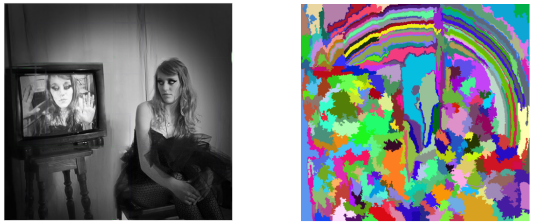
The problem of object localization is the most difficult part of object detection. One approach is that we use sliding window of different size to locate objects in the image. This approach is called Exhaustive search. This approach is computationally very expensive as we need to search for object in thousands of windows even for small image size. Some optimization has been done such as taking window sizes in different ratios (instead of increasing it by some pixels). But even after this due to number of windows it is not very efficient. This article looks into selective search algorithm which uses both Exhaustive search and segmentation (a method to separate objects of different shapes in the image by assigning them different colors).

Algorithm Of Selective Search :

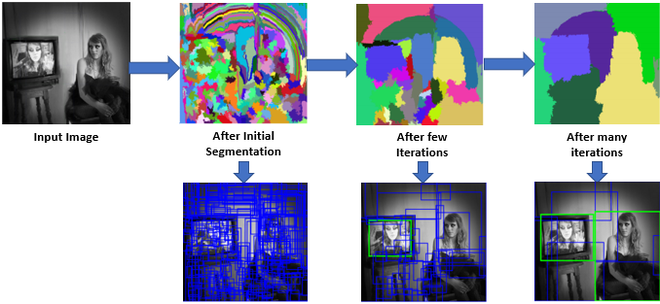
1. Generate initial sub-segmentation of input image using the method describe by Felzenszwalb et al in his paper “Efficient Graph-Based Image Segmentation “.

2. Recursively combine the smaller similar regions into larger ones. We use Greedy algorithm to combine similar regions to make larger regions. The algorithm is written below.

   Greedy Algorithm : 
   
   1. From set of regions, choose two that are most similar.
   2. Combine them into a single, larger region.
   3. Repeat the above steps for multiple iterations.

    

   

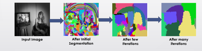
3. Use the segmented region proposals to generate candidate object locations.
   

Similarity in Segmentation:

The selective search paper considers four types of similarity when combining the initial small segmentation into larger ones. These similarities are: 

• Color Similarity : Specifically for each region we generate the histogram of each channels of colors present in image .In this paper 25 bins are taken in histogram of each color channel. This gives us 75 bins (25 for each R, G and B) and all channels are combined into a vector  (n = 75) for each region. Then we find similarity using equation below:
• Texture Similarity : Texture similarity are calculated using generated 8 Gaussian derivatives of image and extracts histogram with 10 bins for each color channels. This gives us 10 x 8 x 3 = 240 dimensional vector for each region. We derive similarity using this equation.
• Size Similarity : The basic idea of size similarity is to make smaller region merge easily. If this similarity is not taken into consideration then larger region keep merging with larger region and region proposals at multiple scales will be generated at this location only.  
• Fill Similarity : Fill Similarity measures how well two regions fit with each other. If two region fit well into one another (For Example one region is present in another) then they should be merged, if two region does not even touch each other then they should not be merged. Now, Above four similarities combined to form a final similarity.

Results :

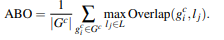
To measure the performance of this method. The paper describes an evaluation parameter known as MABO (Mean Average Best Overlap). There are two version of selective search came Fast and Quality. The difference between them is Quality generated much more bounding boxes than Fast and so takes more time to compute but have higher recall and ABO(Average Best Overlap) and MABO (Mean Average Best overlap). We calculated ABO as follows.

As we can observe that when all the similarities are used in combination, It gives us best MABO. However, it can also be conclude RGB is not best color scheme to use in this method. HSV, Lab and rgI all performs better than RGB, this is because these are not sensitive to shadows and brightness changes. 

But when we diversify and combine these different similarities, color scheme and threshold values (k),

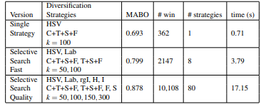
In selective search paper, it applies greedy method based on MABO on different strategies to get above results. We can say that this method of combining different strategies although gives better MABO, but the run time also increases considerably.

Selective Search In Object Recognition :

In selective search paper, authors use this algorithm on object detection and train a model using by giving ground truth examples and sample hypothesis that overlaps 20-50% with ground truth(as negative example) into SVM classifier and train it to identify false positive . The architecture of model used in given below.

The result generated on VOC 2007 test set is,

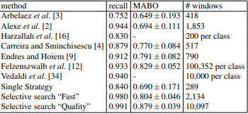
As we can see that it produces a very high recall and best MABO on VOC 2007 test Set and it requires much less number of windows to be processed as compared to other algorithms who achieve similar recall and MABO.

 

Applications :

Selective Search is widely used in early state-of-the-art architecture such as R-CNN, Fast R-CNN etc. However, Due to number of windows it processed, it takes anywhere from 1.8 to 3.7 seconds (Selective Search Fast) to generate region proposal which is not good enough for a real-time object detection system. 

 

Reference:

• Selective Search paper (Selective Search for Object Detection)
• Stanford Computer Vision Slides