Simpson’s Rule in MATLAB
Last Updated :
17 Dec, 2021
Simpson’s 1/3 rule is a numerical method used for the evaluation of definite integrals. MATLAB does not provide an in-built function to find numerical integration using Simpson’s rule. However, we can find that using the below formula.
The formula for numerical integration using Simpson’s rule is:
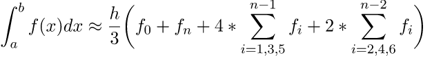
where, h = (b-a)/n
In Simpson’s 1/3 rule, we evaluate the definite integral using integration by successive segments of the curve. It helps us to make the approximations more precise as compared to trapezoidal rule where straight lines segments were used instead of parabolic arcs.
Note: For Simpson’s 1/3 Rule, n must be even.
Example: Evaluate  within limit 4 to 5.2
Matlab
syms x
a = 4;
b = 5.2;
n = 6;
f1 = log(x);
f = inline(f1);
h = (b - a)/n;
X = f(a)+f(b);
Odd = 0;
Even = 0;
for i = 1:2:n-1
xi=a+(i*h);
Odd=Odd+f(xi);
end
for i = 2:2:n-2
xi=a+(i*h);
Even=Even+f(xi);
end
I = (h/3)*(X+4*Odd+2*Even);
disp('The approximation of above integral is: ');
disp(I);
|
Output:

Like Article
Suggest improvement
Share your thoughts in the comments
Please Login to comment...