Unconstrained Multivariate Optimization

Last Updated : 17 Jul, 2020

Wikipedia defines optimization as a problem where you maximize or minimize a real function by systematically choosing input values from an allowed set and computing the value of the function. That means when we talk about optimization we are always interested in finding the best solution. So, let say that one has some functional form(e.g in the form of f(x)) and he is trying to find the best solution for this functional form. Now, what does best mean? One could either say he is interested in minimizing this functional form or maximizing this functional form.
Generally, an optimization problem has three components.

minimize f(x),
w.r.t x ,
subject to a < x < b

where, f(x) : Objective function
x : Decision variable
a < x < b : Constraint

What’s a multivariate optimization problem? In a multivariate optimization problem, there are multiple variables that act as decision variables in the optimization problem.

z = f(x₁,x₂,x₃…..x_n)

So, when you look at these types of problems a general function z could be some non-linear function of decision variables x₁,x₂,x₃ to x_n. So, there are n variables that one could manipulate or choose to optimize this function z. Notice that one could explain univariate optimization using pictures in two dimensions that is because in the x-direction we had the decision variable value and in the y-direction, we had the value of the function. However, if it is multivariate optimization then we have to use pictures in three dimensions and if the decision variables are more than 2 then it is difficult to visualize. What’s unconstrained multivariate optimization? As the name suggests multivariate optimization with no constraints is known as unconstrained multivariate optimization. Example:

min f(x̄)
w.r.t x̄
x̄ ∈ Rⁿ

So, when you look at this optimization problem you typically write it in this above form where you say you are going to minimize f(x̄), and this function is called the objective function. And the variable that you can use to minimize this function which is called the decision variable is written below like this w.r.t x̄ here and you also say x̄ is continuous that is it could take any value in the real number line.

The necessary and sufficient conditions for x̄^* to be the minimizer of the function f(x̄^*)

In case of multivariate optimization the necessary and sufficient conditions for x̄^* to be the minimizer of the function f(x̄) are:
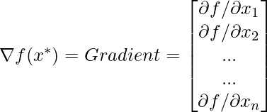
First-order necessary condition: ∇ f(x̄^*) = 0

Second-order sufficiency condition: ∇ ² f(x̄^*) has to be positive definite.
where, $\nabla f(x^*) = Gradient = \begin{bmatrix} \partial f/ \partial x_1\\ \partial f/ \partial x_2\\ ...\\ ...\\ \partial f/ \partial x_n\\ \end{bmatrix}$ ,and $\nabla ^2 f(x^*) = Hessian = \begin{bmatrix} \partial ^2f/ \partial x_1^2 & \partial ^2f/\partial x_1 \partial x_2 & ... & \partial ^2f/ \partial x_1 \partial x_n\\ \partial ^2f/\partial x_2 \partial x_1 & \partial ^2f/ \partial x_2^2 & ... & \partial ^2f/ \partial x_2 \partial x_n\\ ... & ... & ... & ...\\ ... & ... & ... & ...\\ \partial ^2f/\partial x_n \partial x_1 & \partial ^2f/\partial x_n \partial x_2 & ... & \partial ^2f/ \partial x_n^2\\ \end{bmatrix}$

Let us quickly solve a numerical example on this to understand these conditions better.

Numerical Example

Problem:
min 

Solution:
According to the first-order condition



By solving the two equation we got value of  and  as



To check whether this is a maximum point or a minimum point, and
to do so we look at the second-order sufficiency condition. 
So according to the second-order sufficiency condition:



And we know that the Hessian matrix is said to be positive definite at a point 
if all the eigenvalues of the Hessian matrix are positive. So now let's find the
eigenvalues of the above Hessian matrix. To find eigenvalue refer here. 
And to find eigenvalue in python refer here.

So the eigenvalue of the above hessian matrix is



So the eigenvalues for this found to be both positive; 
that means, that this is a minimum point.