What is Efficient Programming?
Efficient programming is programming in a manner that, when the program is executed, uses a low amount of overall resources pertaining to computer hardware.
Practicing to create a small file size and low resource algorithm results in an efficient program.
Below are some important concepts you should know to understand efficient
- Space and time When we refer to the efficiency of a program, we aren’t just thinking about its speed—we’re considering both the time it will take to run the program and the amount of space the program will require in the computer’s memory. Often there will be a trade-off between the two, where you can design a program that runs faster by selecting a data structure that takes up more space—or vice versa.
- Algorithms: An algorithm is essentially a series of steps for solving a problem. Usually, an algorithm takes some kind of input (such as an unsorted list) and then produces the desired output (such as a sorted list).
Quantifying Efficiency:
It’s fine to say “this algorithm is more efficient than that algorithm”, but can we be more specific than that? Can we quantify things and say how much more efficient the algorithm is?
Let’s look at a simple example so that we have something specific to consider. Here is a short (and rather silly) function written in Python:
Example:
Choice 1:
C++
#include <iostream>
int some_function(int n) {
for (int i = 0; i < 2; ++i) {
n += 100;
}
return n;
}
int main() {
int result = some_function(50);
std::cout << "Result: " << result << std::endl;
return 0;
}
|
Java
public class Main {
static int someFunction(int n) {
for (int i = 0; i < 2; ++i) {
n += 100;
}
return n;
}
public static void main(String[] args) {
int result = someFunction(50);
System.out.println("Result: " + result);
}
}
|
Python3
def some_function(n):
for i in range(2):
n += 100
return n
|
C#
using System;
class Program
{
static int SomeFunction(int n)
{
for (int i = 0; i < 2; ++i)
{
n += 100;
}
return n;
}
static void Main(string[] args)
{
int result = SomeFunction(50);
Console.WriteLine("Result: " + result);
}
}
|
Javascript
function SomeFunction(n) {
for (let i = 0; i < 2; ++i) {
n += 100;
}
return n;
}
function main() {
let result = SomeFunction(50);
console.log("Result: " + result);
}
main();
|
What does it do?
- Adds 2 to the given input
- Adds 100 to the given input
- Adds 200 to the given input
Solution: 3. Adds 200 to the given input.
Choice 2:
Python3
def other_function(n):
for i in range(100):
n += 2
return n
|
What does it do?
- Adds 2 to the given input
- Adds 100 to the given input
- Adds 200 to the given input
Although the two functions have the exact same end result, one of them iterates many times to get to that result, while the other iterates only a couple of times. This was admittedly a rather impractical example (you could skip the for loop altogether and just add 200 to the input), but it nevertheless demonstrates one way in which efficiency can come up.
Counting lines to quantify Efficiency:
With the above examples, what we basically did was count the number of lines of code that were executed. Let’s look again at the first function:
Python3
def some_function(n):
for i in range(2):
n += 100
return n
|
There are four lines in total, but the line inside the for loop will run twice. So running this code will involve running 5 lines.
Now let’s look at the second example:
Python3
def other_function(n):
for i in range(100):
n += 2
return n
|
In this case, the code inside the loop runs 100 times. So running this code will involve running 103 lines!
Note: Counting lines of code is not a perfect way to quantify efficiency, and we’ll see that there’s a lot more to it as we go through the program. But in this case, it’s an easy way for us to approximate the difference in efficiency between the two solutions.
We can see that if a language has to perform an “addition” operation 100 times, this will certainly take longer than if it only has to perform an addition operation twice!
Input size and Efficiency:
Let us have a look at the following function:
Python3
def some_function(n):
for i in range(2):
n += 100
return n
|
Suppose we call this function and give it the value 1, like this:
And then we call it again, but give it the input 1000:
Will this change the number of lines of code that get run?
No — the same number of lines will run in both cases.
Now take a look at the following function:
Python3
def say_GeeksforGeeks(n):
for i in range(n):
print("GeeksforGeeks !")
|
Suppose we call it like this:
And then we call it like this:
Will this change the number of lines of code that get run?
Yes — GeeksforGeeks(1000) will involve running more lines of code.
This highlights a key idea: As the input to an algorithm increases, the time required to run the algorithm may also increase.
Rate of increase to measure Efficiency:
One other, approach to measure efficiency is measuring rate of increase of time. Some most common relations are mentioned below:
Linear Relationship:
Python3
def say_GeeksforGeeks(n):
for letters in range(n):
print("GeeksforGeeks !")
|
When we increase the size of the input n by 1, how many more lines of code get run? When n goes up by 1, the number of lines run also goes up by 1.
We can say that as the input increases, the number of lines executed increases by a proportional amount. Any change in the input is tied to a consistent, proportional change in the number of lines executed. This type of relationship is called a linear relationship. Below is the graph for this relationship.
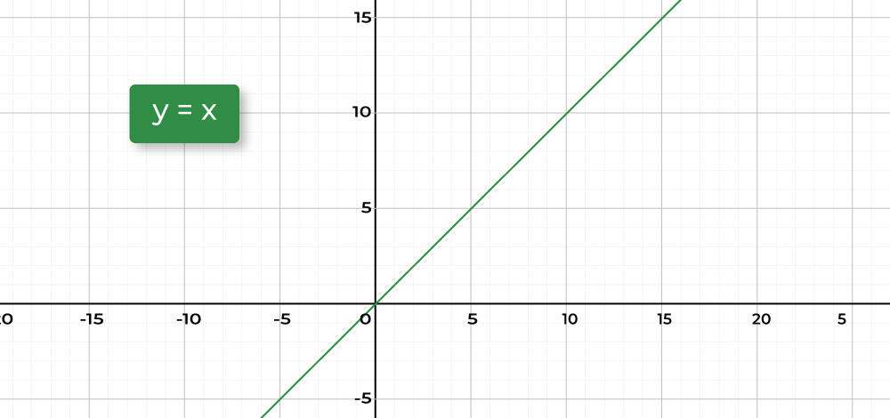
Linear Relationship
The horizontal axis, n, represents the size of the input (in this case, the number of times we want to print “GeeksforGeeks!”). The vertical axis, N, represents the number of operations that will be performed. In this case, we’re thinking of an “operation” as a single line of code (which is not the most accurate, but it will do for now). We can see that if we give the function a larger input, this will result in more operations. And we can see the rate at which this increase happens. The rate of increase is linear.
Quadratic Relationship:
Now here’s a slightly modified version of the say_GeeksforGeeks() function:
Python3
def say_GeeksforGeeks(n):
for i in range(n):
for i in range(n):
print("GeeksforGeeks !")
|
Notice that it has a nested loop. Looking at the say_GeeksforGeeks() function from the above exercise, what can we say about the relationship between the input, n, and the number of times the function will print “GeeksforGeeks!“?
The function will print the word exactly n2 times. Notice that when the input goes up by a certain amount, the number of operations goes up by the square of that amount. This is what we would call a quadratic rate of increase. Let’s compare that with the linear rate of increase. Below is the Graph showing linear and quadratic relationships.
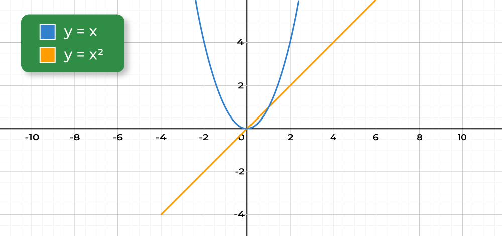
Relation between Linear and Quadratic Relationship
Our code with the nested for loop exhibits the quadratic relationship on the left. Notice that this results in a much faster rate of increase. As we ask our code to print larger and larger numbers of “GeeksforGeeks!”, the number of operations the computer has to perform shoots up more quickly than the other which shows a linear increase.
This brings us to a second key point. We can add it to what we said earlier:
As the input to an algorithm increases, the time required to run the algorithm may also increase and different algorithms may increase at different rates.
We’ve looked here only at a couple of different rates – linear and quadratic. But there are many other possibilities. Here we’ll show some of the common types of rates that come up when designing algorithms.
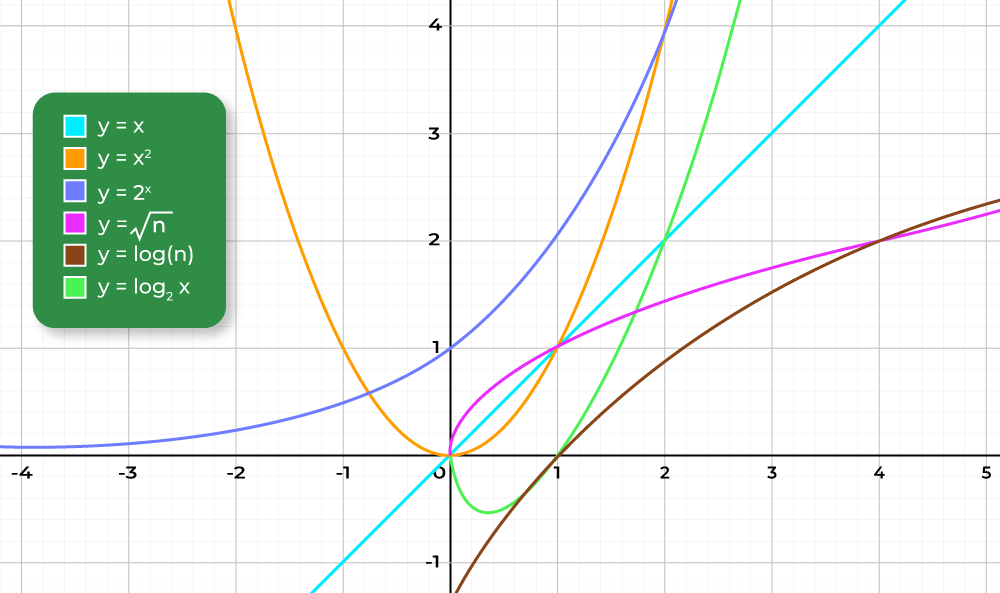
Different Functional Relationships
Note: The rate of increase of an algorithm is also referred to as the order of the algorithm.
References:
- Analysis of Algorithms.
- Intro to CS in Python
Like Article
Suggest improvement
Share your thoughts in the comments
Please Login to comment...