XGBoost is an optimized distributed gradient boosting library designed for efficient and scalable training of machine learning models. It is an ensemble learning method that combines the predictions of multiple weak models to produce a stronger prediction. XGBoost stands for “Extreme Gradient Boosting” and it has become one of the most popular and widely used machine learning algorithms due to its ability to handle large datasets and its ability to achieve state-of-the-art performance in many machine learning tasks such as classification and regression.
One of the key features of XGBoost is its efficient handling of missing values, which allows it to handle real-world data with missing values without requiring significant pre-processing. Additionally, XGBoost has built-in support for parallel processing, making it possible to train models on large datasets in a reasonable amount of time.
XGBoost can be used in a variety of applications, including Kaggle competitions, recommendation systems, and click-through rate prediction, among others. It is also highly customizable and allows for fine-tuning of various model parameters to optimize performance.
XgBoost stands for Extreme Gradient Boosting, which was proposed by the researchers at the University of Washington. It is a library written in C++ which optimizes the training for Gradient Boosting.
Before understanding the XGBoost, we first need to understand the trees especially the decision tree:
Decision Tree:
A Decision tree is a flowchart-like tree structure, where each internal node denotes a test on an attribute, each branch represents an outcome of the test, and each leaf node (terminal node) holds a class label.
A tree can be “learned” by splitting the source set into subsets based on an attribute value test. This process is repeated on each derived subset in a recursive manner called recursive partitioning. The recursion is completed when the subset at a node all has the same value of the target variable, or when splitting no longer adds value to the predictions.
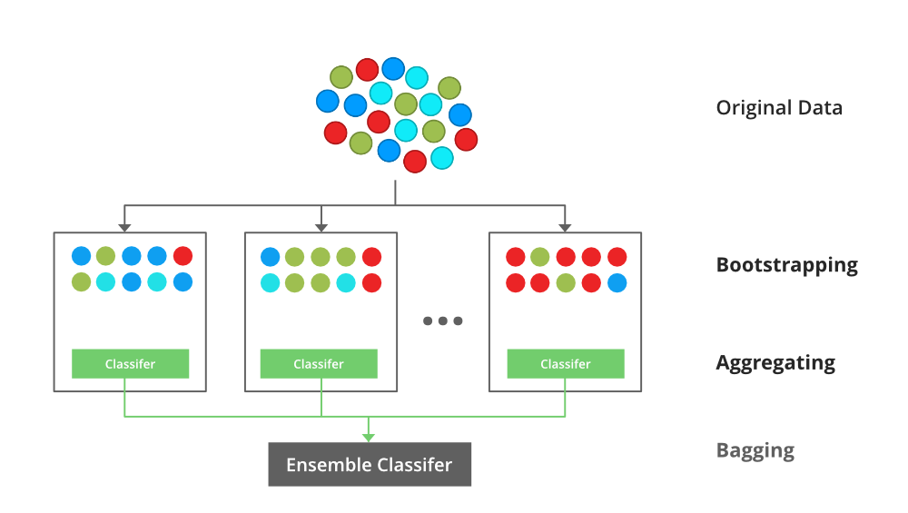
Bagging:
A Bagging classifier is an ensemble meta-estimator that fits base classifiers each on random subsets of the original dataset and then aggregate their individual predictions (either by voting or by averaging) to form a final prediction. Such a meta-estimator can typically be used as a way to reduce the variance of a black-box estimator (e.g., a decision tree), by introducing randomization into its construction procedure and then making an ensemble out of it.
Each base classifier is trained in parallel with a training set which is generated by randomly drawing, with replacement, N examples(or data) from the original training dataset, where N is the size of the original training set. The training set for each of the base classifiers is independent of each other. Many of the original data may be repeated in the resulting training set while others may be left out.
Bagging reduces overfitting (variance) by averaging or voting, however, this leads to an increase in bias, which is compensated by the reduction in variance though.
Bagging classifier
Random Forest:
Every decision tree has high variance, but when we combine all of them together in parallel then the resultant variance is low as each decision tree gets perfectly trained on that particular sample data and hence the output doesn’t depend on one decision tree but multiple decision trees. In the case of a classification problem, the final output is taken by using the majority voting classifier. In the case of a regression problem, the final output is the mean of all the outputs. This part is Aggregation.
The basic idea behind this is to combine multiple decision trees in determining the final output rather than relying on individual decision trees.
Random Forest has multiple decision trees as base learning models. We randomly perform row sampling and feature sampling from the dataset forming sample datasets for every model. This part is called Bootstrap.
Boosting:
Boosting is an ensemble modelling, technique that attempts to build a strong classifier from the number of weak classifiers. It is done by building a model by using weak models in series. Firstly, a model is built from the training data. Then the second model is built which tries to correct the errors present in the first model. This procedure is continued and models are added until either the complete training data set is predicted correctly or the maximum number of models are added.
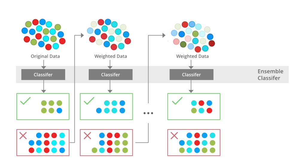
Boosting
Gradient Boosting
Gradient Boosting is a popular boosting algorithm. In gradient boosting, each predictor corrects its predecessor’s error. In contrast to Adaboost, the weights of the training instances are not tweaked, instead, each predictor is trained using the residual errors of predecessor as labels.
There is a technique called the Gradient Boosted Trees whose base learner is CART (Classification and Regression Trees).
XGBoost
XGBoost is an implementation of Gradient Boosted decision trees. XGBoost models majorly dominate in many Kaggle Competitions.
In this algorithm, decision trees are created in sequential form. Weights play an important role in XGBoost. Weights are assigned to all the independent variables which are then fed into the decision tree which predicts results. The weight of variables predicted wrong by the tree is increased and these variables are then fed to the second decision tree. These individual classifiers/predictors then ensemble to give a strong and more precise model. It can work on regression, classification, ranking, and user-defined prediction problems.
Mathematics behind XgBoost
Before beginning with mathematics about Gradient Boosting, Here’s a simple example of a CART that classifies whether someone will like a hypothetical computer game X. The example of tree is below:
The prediction scores of each individual decision tree then sum up to get If you look at the example, an important fact is that the two trees try to complement each other. Mathematically, we can write our model in the form

where, K is the number of trees, f is the functional space of F, F is the set of possible CARTs. The objective function for the above model is given by:

where, first term is the loss function and the second is the regularization parameter. Now, Instead of learning the tree all at once which makes the optimization harder, we apply the additive stretegy, minimize the loss what we have learned and add a new tree which can be summarised below:

The objective function of the above model can be defined as:

![obj^{(t)} = \sum_{i=1}^n (y_{i} - (\hat{y}_{i}^{(t-1)} + f_t(x_i)))^2 + \sum_{i=1}^t\Omega(f_i) \\ = \sum_{i=1}^n [2(\hat{y}_i^{(t-1)} - y_i)f_t(x_i) + f_t(x_i)^2] + \Omega(f_t) + constant](https://www.geeksforgeeks.org/wp-content/ql-cache/quicklatex.com-23480bc3ad2358881c94b6d2663d4146_l3.png "Rendered by QuickLaTeX.com")
Now, let’s apply taylor series expansion upto second order:
![obj^{(t)} = \sum_{i=1}^{n} [l(y_i, \hat{y}_i^{(t-1)}) + g_i f_t(x_i) + \frac{1}{2} h_{i} f_{t}^2(x_i)] + \Omega(f_t) + constant](https://www.geeksforgeeks.org/wp-content/ql-cache/quicklatex.com-736f172f2a3f21cbbab8181397f1f074_l3.png "Rendered by QuickLaTeX.com")
where g_i and h_i can be defined as:

Simplifying and removing the constant:
![\sum_{i=1}^n [g_{i} f_{t}(x_i) + \frac{1}{2} h_{i} f_{t}^2(x_i)] + \Omega(f_t)](https://www.geeksforgeeks.org/wp-content/ql-cache/quicklatex.com-d124d55ef910d3f55fcd701ffb2ba8a2_l3.png "Rendered by QuickLaTeX.com")
Now, we define the regularization term, but first we need to define the model:

Here, w is the vector of scores on leaves of tree, q is the function assigning each data point to the corresponding leaf, and T is the number of leaves. The regularization term is then defined by:

Now, our objective function becomes:
![obj^{(t)} \approx \sum_{i=1}^n [g_i w_{q(x_i)} + \frac{1}{2} h_i w_{q(x_i)}^2] + \gamma T + \frac{1}{2}\lambda \sum_{j=1}^T w_j^2\\ = \sum^T_{j=1} [(\sum_{i\in I_j} g_i) w_j + \frac{1}{2} (\sum_{i\in I_j} h_i + \lambda) w_j^2 ] + \gamma T](https://www.geeksforgeeks.org/wp-content/ql-cache/quicklatex.com-6b829944377420f6f97bf496b0ff365e_l3.png "Rendered by QuickLaTeX.com")
Now, we simplify the above expression:
![obj^{(t)} = \sum^T_{j=1} [G_jw_j + \frac{1}{2} (H_j+\lambda) w_j^2] +\gamma T](https://www.geeksforgeeks.org/wp-content/ql-cache/quicklatex.com-abf23bceccd2504e396cdc2b283e3d1b_l3.png "Rendered by QuickLaTeX.com")
where,

In this equation, w_j are independent of each other, the best  for a given structure q(x) and the best objective reduction we can get is:

where, \gamma is pruning parameter, i.e the least information gain to perform split.
Now, we try to measure how good the tree is, we can’t directly optimize the tree, we will try to optimize one level of the tree at a time. Specifically we try to split a leaf into two leaves, and the score it gains is
![Gain = \frac{1}{2} \left[\frac{G_L^2}{H_L+\lambda}+\frac{G_R^2}{H_R+\lambda}-\frac{(G_L+G_R)^2}{H_L+H_R+\lambda}\right] - \gamma](https://www.geeksforgeeks.org/wp-content/ql-cache/quicklatex.com-45ae40ccc92894f882cbbe992f87efcc_l3.png "Rendered by QuickLaTeX.com")
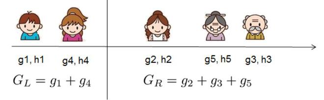
Calculation of Information Gain
Examples
Let’s consider an example dataset:
| Years of Experience | Gap | Annual salary (in 100k) |
|---|
| 1 | N | 4 |
| 1.5 | Y | 4 |
| 2.5 | Y | 5.5 |
| 3 | N | 7 |
| 5 | N | 7.5 |
| 6 | N | 8 |
- First we take the base learner, by default the base model always take the average salary i.e
 (100k). Now, we calculate the residual values:
| Years of Experience | Gap | Annual salary (in 100k) | Residuals |
|---|
| 1 | N | 4 | -2 |
| 1.5 | Y | 4 | -2 |
| 2.5 | Y | 5.5 | -0.5 |
| 3 | N | 7 | 1 |
| 5 | N | 7.5 | 1.5 |
| 6 | N | 8 | 2 |
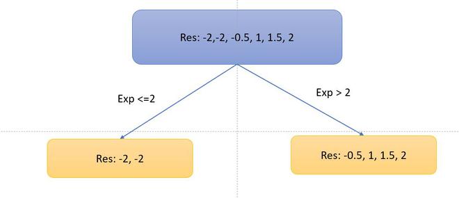
- Now, let’s consider the decision tree, we will be splitting the data based on experience <=2 or otherwise.
- Now, let’s calculate the similarity metrices of left and right side. Since, it is the regression problem the similarity metric will be:

where, \lambda = hyperparameter
and for the classification problem:

where, P_r = probability of either left side of right side. Let’s take  ,the similarity metrics of the left side:
 and for the right side.
 and for the top branch:
 .
.
- Now, the information gain from this split is:

Similarly, we can try multiple splits and calculate the information gain. We will take the split with the highest information gain. Let’s for now take this information gain. Further, we will split the decision tree if there is a gap or not.
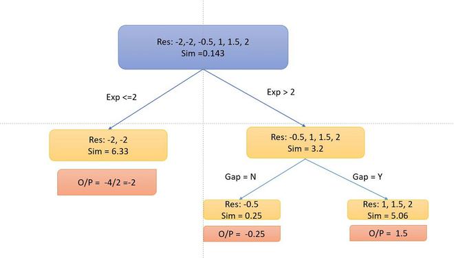
- Now, As you can notice that I didn’t split into the left side because the information Gain becomes negative. So, we only perform split on the right side.
- To calculate the particular output, we follow the decision tree multiplied with a learning rate \alpha (let’s take 0.5) and add with the previous learner (base learner for the first tree) i.e for data point 1: o/p = 6 + 0.5 *-2 =5. So our table becomes.
- Similarly, the algorithm produces more than one decision tree and combine them additively to generate better estimates
Optimization and Improvement
System Optimization:
- Regularization: Since the ensembling of decisions, trees can sometimes lead to very complex. XGBoost uses both Lasso and Ridge Regression regularization to penalize the highly complex model.
- Parallelization and Cache block: In, XGboost, we cannot train multiple trees parallel, but it can generate the different nodes of tree parallel. For that, data needs to be sorted in order. In order to reduce the cost of sorting, it stores the data in blocks. It stored the data in the compressed column format, with each column sorted by the corresponding feature value. This switch improves algorithmic performance by offsetting any parallelization overheads in computation.
- Tree Pruning: XGBoost uses max_depth parameter as specified the stopping criteria for the splitting of the branch, and starts pruning trees backward. This depth-first approach improves computational performance significantly.
- Cache-Awareness and Out-of-score computation: This algorithm has been designed to make use of hardware resources efficiently. This is accomplished by cache awareness by allocating internal buffers in each thread to store gradient statistics. Further enhancements such as ‘out-of-core computing optimize available disk space while handling big data-frames that do not fit into memory. In out-of-core computation, Xgboost tries to minimize the dataset by compressing it.
- Sparsity Awareness: XGBoost can handle sparse data that may be generated from preprocessing steps or missing values. It uses a special split finding algorithm that is incorporated into it that can handle different types of sparsity patterns.
- Weighted Quantile Sketch: XGBoost has in-built the distributed weighted quantile sketch algorithm that makes it easier to effectively find the optimal split points among weighted datasets.
- Cross-validation: XGboost implementation comes with a built-in cross-validation method. This helps the algorithm prevents overfitting when the dataset is not that big,
Advantages Or Disadvantages:
Advantages of XGBoost:
- Performance: XGBoost has a strong track record of producing high-quality results in various machine learning tasks, especially in Kaggle competitions, where it has been a popular choice for winning solutions.
- Scalability: XGBoost is designed for efficient and scalable training of machine learning models, making it suitable for large datasets.
- Customizability: XGBoost has a wide range of hyperparameters that can be adjusted to optimize performance, making it highly customizable.
- Handling of Missing Values: XGBoost has built-in support for handling missing values, making it easy to work with real-world data that often has missing values.
- Interpretability: Unlike some machine learning algorithms that can be difficult to interpret, XGBoost provides feature importances, allowing for a better understanding of which variables are most important in making predictions.
Disadvantages of XGBoost:
- Computational Complexity: XGBoost can be computationally intensive, especially when training large models, making it less suitable for resource-constrained systems.
- Overfitting: XGBoost can be prone to overfitting, especially when trained on small datasets or when too many trees are used in the model.
- Hyperparameter Tuning: XGBoost has many hyperparameters that can be adjusted, making it important to properly tune the parameters to optimize performance. However, finding the optimal set of parameters can be time-consuming and requires expertise.
- Memory Requirements: XGBoost can be memory-intensive, especially when working with large datasets, making it less suitable for systems with limited memory resources.
References:
Like Article
Suggest improvement
Share your thoughts in the comments
Please Login to comment...