Mood’s Median Test
Last Updated :
25 Aug, 2021
Mood’s Median Test: It is a non-parametric alternative to one way ANOVA. It is a special case of Pearson’s Chi-Squared Test. It tests whether the medians of two or more groups differ and also calculates a range of values that is likely to include the difference between population medians. In this test, different data groups have similarly shaped distributions.
Data in each of the samples are assigned to two groups-
- One consisting of data whose values are higher than the combined median of the samples.
- The other consisting of data whose value are at the median or below.
Assumptions of Mood’s Median Test
- Data should include only one categorical factor.
- Response variable should be continuous.
- Sample data need not be normally distributed.
- Sample sizes can be unequal too.
Null and Alternate Hypothesis of Mood’s Median Test
Null Hypothesis: The population Medians are all equal.
Alternate Hypothesis: The Medians are not all equal OR At least 2 of them differ from each other.
H0 : M1 = M2 = M3 = ..... Mk  ; M= Median
H1 : At least two of them show significant difference.
Test Statistic for Mood’s Median Test
Test statistic for this type of test is the Chi=Squared statistic where we look for the Observed and Expected frequencies.
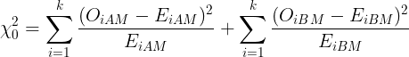
OiAM = Observed Frequencies of ith sample above Median
OiBM = Observed Frequencies of ith sample below Median
EiAM = Expected Frequencies of ith sample above Median
EiBM = Expected Frequencies of ith sample below Median
Rejection Criteria
We reject the Null Hypothesis if Test Statistic X02 is greater than the critical value at a given level of significance (alpha) and k-1 degrees of freedom.
Steps to Perform Mood’s Median Test
Let us take an example to understand how to perform this test.
Example: 35 Students from a City in India were asked to provide ratings for a restaurant chain in different areas of the city. There were 11 Students for Area A, 12 Students for Area B and 12 Students for Area C. The ratings are given on the basis of 4 conditions of cleanliness, taste etc. Each condition can get a maximum of 5 points hence a Restaurant can get a Maximum rating of 20 points. Test whether the Medians are the same for the 3 Restaurant chains. ( alpha = 5%)
| Area A |
Area B |
Area C |
| 17 |
19 |
12 |
| 16 |
15 |
16 |
| 13 |
15 |
18 |
| 10 |
17 |
13 |
| 19 |
16 |
13 |
| 18 |
12 |
15 |
| 16 |
10 |
19 |
| 14 |
19 |
20 |
| 15 |
12 |
11 |
| 17 |
13 |
13 |
| 18 |
14 |
17 |
| |
15 |
18 |
Step 1: Define NULL and Alternate Hypothesis
H0 : MA = MB = MC. M= Median.
H1 : At least two of them differ from each other.
Step 2: State Alpha (Level of Significance)
Alpha = 0.05
Step 3: Calculate Degrees of Freedom
DF = K-1       ; K = number of sample groups.
Here , DF = 3-1 =2.
Step 4: Find out the Critical Chi-Square Value.
Use this table to find out the critical chi-square value for alpha = 0.05 and DF = 2.
X2 = 5.991
Step 5: State Decision Rule
If X02 is greater than 5.991 , reject the Null Hypothesis.
Step 6: Calculate the Overall Median
There are total 35 data entries so the median will be the 18th element after arranging in ascending order.
Arranging in ascending order -
10 10 11 12 12 12 13 13 13 13 13 14 14 15 15 15 15 15
16 16 16 16 17 17 17 17 18 18 18 18 19 19 19 19 20
The overall median is 15
Step 7: Construct a table using the Observed values with two columns – one showing the number of ratings above the overall median for each Area and the other showing the number of ratings below the overall median for each Area.
| Observed |
|
| |
Area A |
Area B |
Area C |
Totals |
| > overall median |
7 |
4 |
6 |
17 |
| <= overall median |
4 |
8 |
6 |
18 |
| Totals |
11 |
12 |
12 |
35 |
Here 7 ratings in Area A are above the overall Median and 4 are below or equal to the overall Median.
Step 8: Construct a similar table of Expected values.
The expected values are obtained by –
(Column total * Row Total) / N     ; N= total number of data entries

Here,  For Area A the Expected value for > overall median will be (11*17)/35 =  5.34
| Expected |
|
| |
Area A |
Area B |
Area C |
Totals |
| > overall median |
5.43 |
5.83 |
5.83 |
17 |
| <= overall median |
5.66 |
6.17 |
6.17 |
18 |
| Totals |
11 |
12 |
12 |
35 |
Step 9: Calculate the Test Statistic

X02 = 2.067
Step 10: State Results
Since X02 is less than 5.991 , We accept the Null Hypothesis.
Step 11: State Conclusion
We can conclude that the Medians are the same for the 3 Restaurant Chains.
This is all about the Mood’s Median Test. For any queries do leave a comment down below.
Share your thoughts in the comments
Please Login to comment...