Quantile Regression in R Programming
Last Updated :
31 Aug, 2020
Quantile Regression is an algorithm that studies the impact of independent variables on different quantiles of the dependent variable distribution. Quantile Regression provides a complete picture of the relationship between Z and Y. It is robust and effective to outliers in Z observations. In Quantile Regression, the estimation and inferences are distribution free. Quantile regression is an extension of linear regression i.e when the conditions of linear regression are not met (i.e., linearity, independence, or normality), it is used. It estimates conditional quantile function as a linear combination of the predictors, used to study the distributional relationships of variables, helps in detecting heteroscedasticity, and also useful for dealing with censored variables. It is very easy to perform quantile regression in R programming.
Mathematical Expression
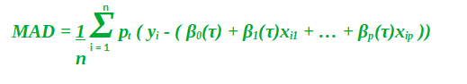
Quantile regression is more effective and robust to outliers. In Quantile regression, you’re not limited to just finding the median i.e you can calculate any percentage(quantile) for a particular value in features variables. For example, if one wants to find the 30th quantile for the price of a particular building, that means that there is a 30% chance the actual price of the building is below the prediction, while there is a 70% chance that the price is above. Therefore, the quantile regression model equation is:

So, now instead of being constants, the beta coefficients have now functioned with a dependency on the quantile. Finding the values for these betas at a particular quantile value has almost the same process as it does for regular linear quantization. We now have to reduce the median absolute deviation.
Also, Mathematically pt takes the form:
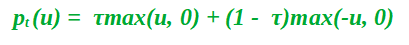
The function pt(u) is the check function which gives asymmetric weights to error which depends on the quantile and the overall sign of the error.
Implementation in R
The Dataset:
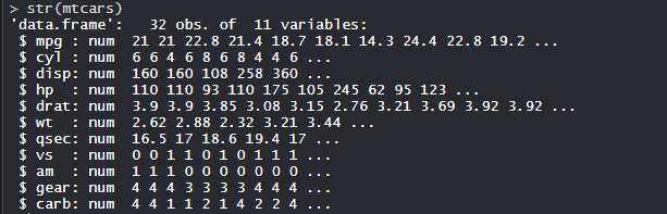
mtcars(motor trend car road test) comprises fuel consumption, performance, and 10 aspects of automobile design for 32 automobiles. It comes pre-installed with dplyr package in R.
R
install.packages("dplyr")
library(dplyr)
str(mtcars)
|
Output:
Performing Quantile Regression on Dataset:
Using the Quantile regression algorithm on the dataset by training the model using features or variables in the dataset.
R
install.packages("quantreg")
install.packages("ggplot2")
install.packages("caret")
library(quantreg)
library(dplyr)
library(ggplot2)
library(caret)
Quan_fit <- rq(disp ~ wt, data = mtcars)
Quan_fit
summary(Quan_fit)
plot(disp ~ wt, data = mtcars, pch = 16, main = "Plot")
abline(lm(disp ~ wt, data = mtcars), col = "red", lty = 2)
abline(rq(disp ~ wt, data = mtcars), col = "blue", lty = 2)
|
Output:
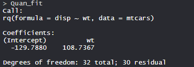
The model Quan_fit has Intercept -129.7880 with 32 Degrees of Freedom.
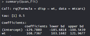
The Model has tau value 0.5 with lower bd is -185.6818 and upper bd is -100.5439 of coefficient -129.7880.
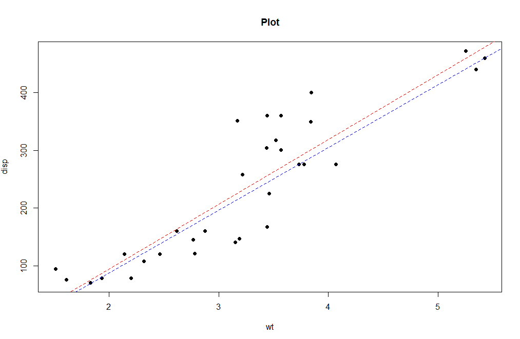
The plot shows the quantile regression line in the Blue and linear regression line in Red. So, Quantile regression applications are used in growth charts, statistics, regression analysis with full capacity.
Advantages of Quantile Regression
- Helps in understanding the relationship between variables of data that have non-linear relationships having predictor variables.
- It is robust and effective for Outliers.
- It helps in obtaining statistical dispersion which helps in deeper review between the relationship of variables.
Share your thoughts in the comments
Please Login to comment...