What is the Glmnet package in R?
Last Updated :
21 Mar, 2023
R is a popular programming language used for statistical computing, machine learning, and data analysis. The Glmnet package in R is a tool used for fitting linear and logistic regression models with L1 and L2 regularization. Regularization is a method for preventing overfitting in models by introducing a penalty term to the objective function. The glmnet package provides an efficient and scalable implementation of this technique, making it a popular choice for machine learning and data science applications.
In data science, a common challenge is to build predictive models that generalize well to new or nonlinear data. Overfitting, which occurs when a model is too complex and fits the training data too closely, can be a significant problem. Regularization is one approach to preventing overfitting, but it can be difficult to implement efficiently in high-dimensional datasets. The Glmnet package offers an effective solution for this problem.
Regularized Regression
A type of regression that adds a penalty term to the cost function to reduce overfitting.
- Lasso Regression: A type of regularized regression that adds an L1 penalty term to the cost function.
- Ridge Regression: A type of regularized regression that adds an L2 penalty term to the cost function.
- Elastic Net Regression: A type of regularized regression that adds both an L1 and L2 penalty term to the cost function.
Code Explanation:
The primary function used in the Glmnet package is “glmnet”, which fits a generalized linear model with regularization. The function takes several arguments, including the response variable (y), the predictor variables (X), and the type of regularization (L1 or L2). The syntax for the function is as follows:
glmnet(X, y, family = "gaussian", alpha = 1, lambda = NULL)
In this syntax, X is the matrix of predictor variables, y is the response variable, and the family specifies the type of response variable (e.g., Gaussian, binomial, Poisson). Alpha specifies the combination of L1 and L2 regularization, with a value of 1 indicating L1 regularization and a value of 0 indicating L2 regularization. Lambda specifies the strength of the regularization penalty.
Example 1
Steps 1: Install the glmnet package in R using the following command:
install.packages("glmnet")
Step 2: Load the glmnet package in R using the following command
Step 3: Load the mtcars datasets
R
data(mtcars)
X <- as.matrix(mtcars[, -1])
y <- mtcars[, 1]
|
Step 3: Fit a regularized regression model using the glmnet function.
The following code fits a Lasso regression model, and the Summary(model) provides information on the fitted model, like the number of non-zero coefficients, the value of the regularization parameter lambda used, and the coefficients themselves.
R
model = glmnet(X, y, family = "gaussian", alpha = 1)
summary(model)
|
Output:
          Length Class     Mode
a0         79    -none-    numeric
beta      790    dgCMatrix S4
df         79    -none-    numeric
dim         2    -none-    numeric
lambda     79    -none-    numeric
dev.ratio  79    -none-    numeric
nulldev     1    -none-    numeric
npasses     1    -none-    numeric
jerr        1    -none-    numeric
offset      1    -none-    logical
call        5    -none-    call
nobs        1    -none-    numeric
Step 4: Plot the model
plot(model) will plot the relationship between the regularization parameter lambda and the estimate coefficients.
R
plot(model, label = TRUE)
|
Output:
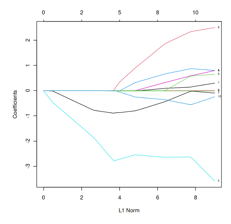
L1 Norm vs Estimated coefficients
In the above graph, each curve represents the path of the coefficients against the L1 norm as lambda varies.
Step 5: Get the model coefficients
Output:
1 x 1 sparse Matrix of class "dgCMatrix"
                     s1
(Intercept) 20.12070307
cyl         -0.21987003
disp         .
hp          -0.01300595
drat         0.77162507
wt          -2.63787681
qsec         0.46074875
vs           0.11747113
am           2.11349978
gear         0.30437026
carb        -0.46452172
Step 6: Prediction
Predict values for new data using the predict function. For example, the following code predicts values for new data using the Lasso regression model:
R
y_pred <- predict(model, X)
|
Example- 2:
- Load the “glmnet” package, which provides functions for fitting regularized linear models.
library(glmnet)
- Load the “mtcars” dataset, which contains information about car models and their performance.
- Create a matrix of predictor variables (X) and a vector of response variables (y) from the mtcars dataset.
- Fit a LASSO model (alpha = 1) with cross-validation using the “cv.glmnet” function, nfolds = 5 specifies the number of cross-validation folds to use.
- Get the summary using the summary(model)
R
library(glmnet)
data(mtcars)
X <- as.matrix(mtcars[, -1])
y <- mtcars[, 1]
fit <- cv.glmnet(X, y, alpha = 1, nfolds = 5)
summary(fit)
|
Output:
           Length Class  Mode
lambda     79     -none- numeric
cvm        79     -none- numeric
cvsd       79     -none- numeric
cvup       79     -none- numeric
cvlo       79     -none- numeric
nzero      79     -none- numeric
call        5     -none- call
name        1     -none- character
glmnet.fit 12     elnet  list
lambda.min  1     -none- numeric
lambda.1se  1     -none- numeric
index       2     -none- numeric
Plot the cross-validation results using the “plot” function.
.png)
cross-validation
Predict the response variable and Plot the Actual vs Predicted graph.
R
y_pred <- predict(fit, X)
plot(y,y_pred,
xlab = 'Actual',
ylab = 'Predicted',
main = 'Actual vs Predicted')
|
Output:

Actual (y) vs predicted
Refer this google colab for entire code.
Share your thoughts in the comments
Please Login to comment...